CS-330 Lecture 8: Variational Inference
This lecture is part of the CS-330 Deep Multi-Task and Meta Learning course, taught by Chelsea Finn in Fall 2023 at Stanford. This post will talk about variational inference, which is a way of approximating complex distributions through Bayesian inference. We will go from talking about latent variable models all the way to amortized variational inference!
Lars Quaedvlieg ·
This post will talk about variational inference, which is a way of approximating complex distributions through Bayesian inference. We will go from talking about latent variable models all the way to amortized variational inference! If you missed the previous post, which was about automatic task construction for unsupervised meta learning, you can head over here to view it.
The link to the lecture slides can be found here.
This lecture is taught in order to be able to discuss Bayesian meta learning in the next part of the series. However, it is a bit different from the rest of the content, so feel free to skip it if you’re already comfortable with this topic!
Probabilistic models
Machine learning is all about probabilistic models! In supervised learning, we try to learn a distribution over a target variable using data from . This conditional distribution depends on the assumptions that you make about this target variable . For example, in classification, you might treat as a categorical variable, which means that comes from a discrete categorical distribution. However, we also often assume that comes from a Gaussian distribution. Note that instead of outputting a single value for , out model predicts the distribution .
The previous two examples are very common, but simple, distributions. For some problems, more complex distributions are necessary in order to formulate the problem effectively. As we will see later on, variational inference will allow us to find solutions for these complex distributions!
First, let’s also very quickly discuss some terminology. Using Bayes’ rule, we have the following equation for a parameter and some evidence :
In this equation,
- is called the posterior distribution. It is the probability after the evidence is considered.
- is called the prior distribution. It is the probability before the evidence is considered.
- is called the likelihood. It is the probability of the evidence, given that is true.
- is called the marginal. It is the probability of the evidence under any circumstance.
The process of training probabilistic models comes from this idea of likelihood. Given that we observe some data , we want to learn the data distribution . However, we will consider a parameterized form . The goal becomes to maximize the likelihood of observing the samples in given :
This assumes independence . One more trick: Since the -function is a monotonically increasing function, we can rewrite this objective function without changing the optimal parameters :
This will help a lot, since we got rid of the long chain of multiplications, which could be catastrophic for gradient-based optimization methods. This method is fundamental to statistics, and is called maximum likelihood estimation.
For simple distributions, such as the categorical and Gaussian distributions that we saw, there are closed-form evaluations of this function. The maximum likelihood estimate of the categorical distribution results in the cross-entropy loss, and the one for the Gaussian distributions is the mean-squared error loss.
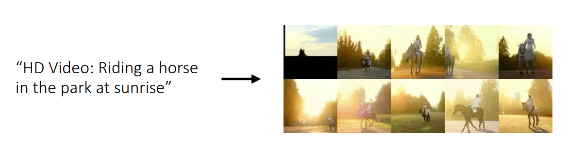
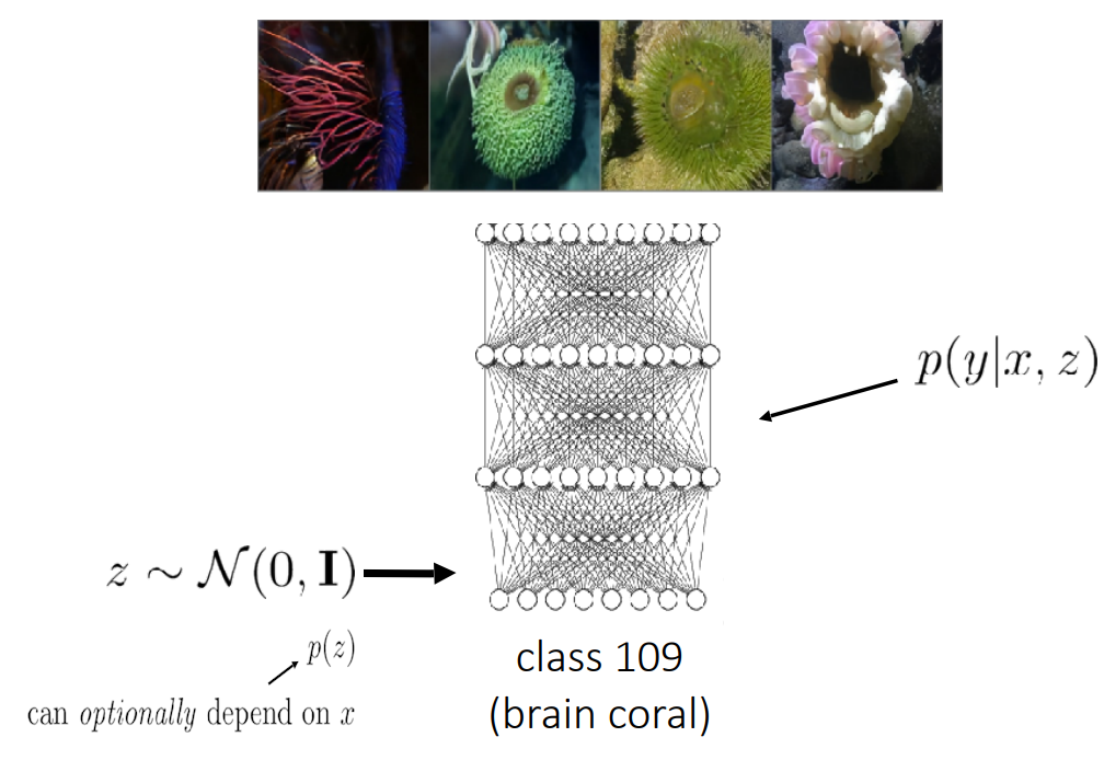
For some problems, assuming the data comes from these distributions is just too simple. For example, generative models over images, text, video, or other data may need a more complex distribution. An example of a text-to-video use-case is depicted above [1]. For this, a Gaussian distribution might just be too simple. Another example is the class of problems that require a multimodal distribution.
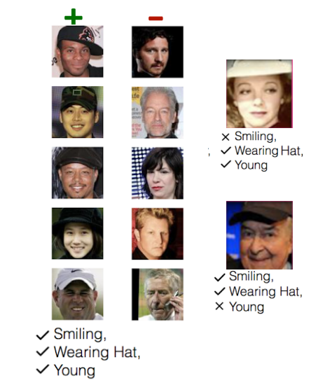
For meta learning, we are so far using a deterministic (i.e. point estimate) of the distribution $p(\phi_i\vert \mathcal{D}^\mathrm{tr}_i, \theta)$. This could be a problem when few-shot learning problems are ambiguous. One example is depicted in the figure on the right. Depending on the representation that the model learns, a point estimate might either learn to distinguish samples based on their youth or whether they are smiling. The goal is ambiguous from the training dataset on the left. Therefore, it would be nice to learn to generate hypotheses by sampling from $p(\phi_i\vert \mathcal{D}^\mathrm{tr}_i, \theta)$. This can be important for safety-critical few-shot learning, learning to active learn [2], and learning how to explore in meta reinforcement learning.
The main question of this lecture: Can we model and train more complex distributions? We will use variational inference to answer this question!
Latent variable models
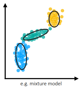
Before we get into variational inference, we will talk about what latent variable models are. We will start by using a few examples and building out the idea. Let’s say we are given the data from $p(x)$ in the right figure. As you can see, fitting a Gaussian distribution would not work very well in this case.
One common method to model these “clustered” points is by using a Gaussian mixture model. The distribution of such a model follows the following formula:
In this distribution, we introduce latent (hidden) variables . In this example, we let be a normal distribution, and be a discrete categorical distribution. Notice that in this case, the latent variables model the clusters that datapoints belong to, and the conditional distribution treats each individual cluster as a normal distribution. Since is a distribution, a datapoint can be part of a mixture of those gaussian distributions, hence the name of the model.
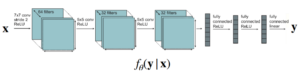
Furthermore, this is also possible for conditional distributions, i.e.:
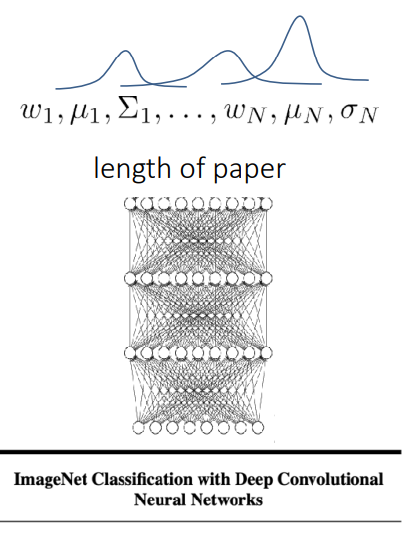
This has the name mixture density network. An example of such a network is shown on the right. Notice that the model outputs the parameters of the distributions instead of a direct value of $y$, which is the length of the paper in this case.
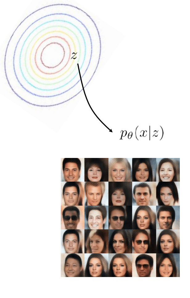
Now that we have seen some examples, let’s generalize it to continuous distributions. Let's observe the equation below:
$$ p(x) = \int p(x\vert z)p(z)dz\;. $$
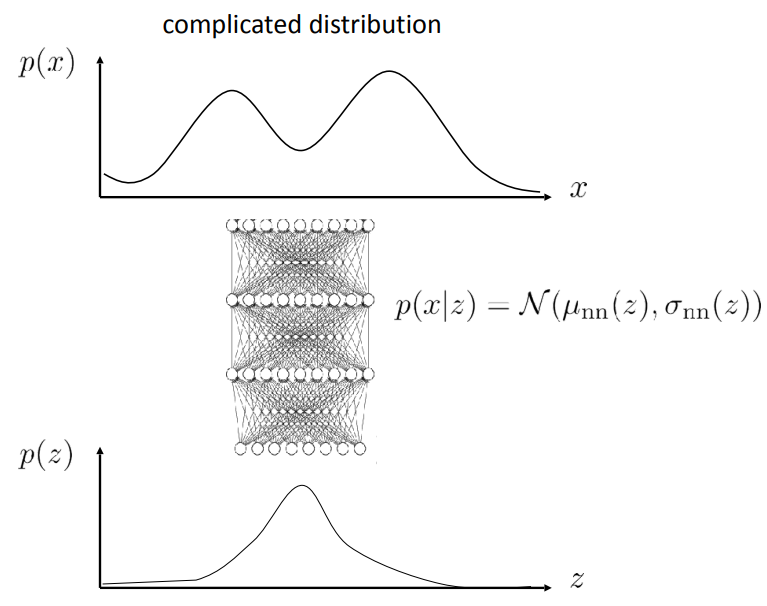
The core idea stays the same: represent a complex distribution by composing two simple distributions. More often than not, $p(x\vert z)$ and $p(z)$ will both be represented as normal distributions.
As you can see in the right figure, we need to sample from $p(z)$ in order to get a sample from $p(x\vert z)$.
However, now, a few questions arise:
-
How can we generate a sample from after the model is trained?
Answer: As we said before, you need to sample a $z$ and then use it to compute $p(x \vert z)$, which you then sample from.
-
How do we evaluate the likelihood of a given sample (e.g. )?
Answer: To compute $p(x_i)$, we need to sample many $z$ from the distribution $p(z)$ in order to get a good approximation of the integral that defines the distribution $p(x) = \int p(x\vert z)p(z)dz$.
Now that we know how to evaluate and sample from latent variable models, let’s look into how we can train these models. Rewriting the maximum likelihood objective with the latent variable model, we obtain the objective function below:
In order to optimize this, we need to find the gradient of this objective. However, the integral in the logarithm is intractable, since it usually does not have a nice closed-form expression, in contrary to the simple distributions we have seen before. Approximating the integral by sampling from is incredibly inefficient.
There exist many papers that use latent variable models, and most of them have (slightly) different ways of training them:
- Generative adversarial networks (GANs) [3]
- Variation autoencoders (VAEs) [4]
- Normalizing flow models [5]
- Diffusion models [6]
Note that autoregressive models do not use latent variables, and we model the target as a categorical distribution, which has the closed-form cross-entropy objective as maximum likelihood estimator.
In this lecture, we will focus on methods that use variational inference. They have a number of benefits and are probably the most common methods to train latent variable models.
Variational inference
In this section, we will introduce variational inference, which is a way of formulating a lower bound on the log-likelihood objective. Furthermore, since we will be optimizing this lower bound, we will look into the tightness of the bound.
We will look at an alternative formulation of the log-likelihood objective, which is called the expected log-likelihood:
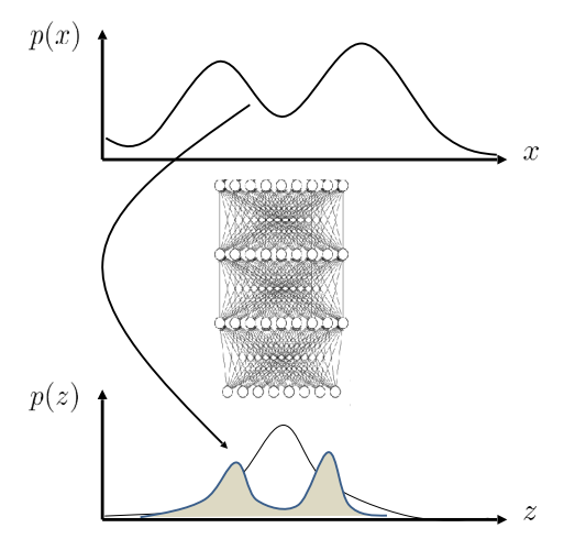
It is very similar to what we have seen, but now we sample the latent variable with $p(z\vert x_i)$ to evaluate the logarithm of the joint distribution $p_\theta(x_i, z)$. The intuition behind this formula is that we can make an educated guess of $z$ by using $p(z\vert x_i)$ instead of doing random sampling from $p(z)$. In the figure on the right, this can be seen as mapping $x_i$ back to the latent distribution $p(z)$.
However, there is a problem. Unfortunately, we do not have access to the distribution $p(z \vert x_i)$. Therefore, we will try to approximate this distribution with the variational distribution $q_i(z) := \mathcal{N}(\mu_i, \sigma_i)$. Note that this is just an estimate, and it will not perfectly model the distribution, but it will help with quickly optimizing the objective function, since we can find likely latent variables given the samples!
Let’s try to now bound and introduce !
In the equation above, we just introduced by adding the fraction , since it equals . Then, we simple rewrote it as an expectation over instead of . This is much nicer than before, since we can actually compute this expectation instead of evaluating an integral. Then, we used Jensen’s inequality to get a lower bound on the objective. We finally did some simple algebra to simplify it. Note that is the entropy function. This bound is called the evidence lower-bound (ELBO).
Let’s spend time to talk about the intuition behind this bound. Since it forms a lower-bound on the original objective, maximizing the ELBO will also maximize the towards the optimal value of original objective. However, there might be some gap, but we will discuss this later on.
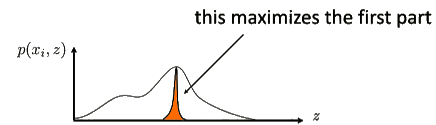
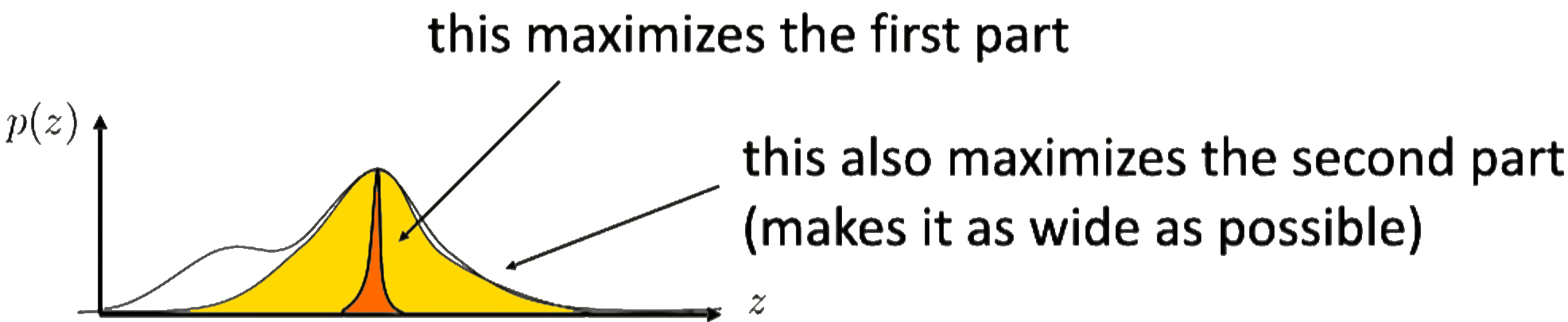
The term $\mathbb{E}_{z \sim q_i}\left[\log p(x_i \vert z) + \log p(z)\right]$ essentially tries to maximize the probability $p(x_i, z)$ for a given $z$. This is highlighted on the figure in the right.
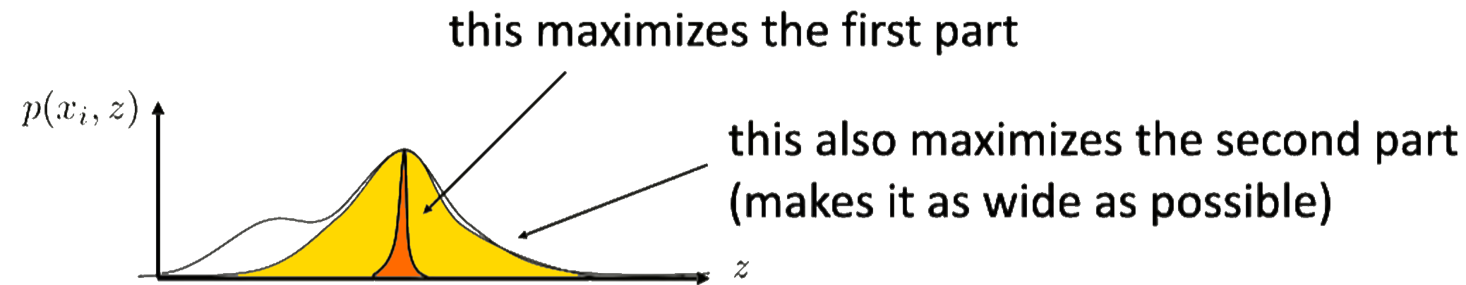
The second term then tries to maximize the entropy $\mathcal{H}(q_i(z))$. Since the entropy is a measure of randomness (e.g. a high entropy corresponds to a high randomness), this term will try to make the fit as random as possible. you can see this as the yellow part in the figure on the right.
Hopefully this gives some intuition behind the objective!
Kullback–Leibler divergence
Let’s take a brief detour and talk about a divergence called the Kullback–Leibler (KL) divergence. It is a divergence between two distributions, and it can be denoted by the following equation:
It can be seen as a difference between distributions. But, in the last line, you can see that it also measures how small the expected log probability of under distribution , minus the entropy of . We will again build some intuition on this.
However, note that we are minimizing the KL-divergence, since we want the distributions to be as similar as possible. In this case, we are maximizing the log probability under the other distribution, and we are also maximizing the entropy, which will lead to a similar intuition as we saw previously on the ELBO.
Tightness of the lower bound
Now that you have seen the similarities between the KL divergence and the ELBO objectives, let’s try to put them together. We will try to do this by rewriting the KL divergence and uncovering the ELBO objective function. Recall that the ELBO objective is
Further recall that we approximated earlier in order to be able to sample , since we do not have access to . Intuitively, it makes sense that we want to be as close as possible to . Let’s now compute the KL divergence between these distributions to see how well approximates.
From the first to the second line, we use that . Then, from the second to third line, we simplify using the rules of the logarithm and already substitute in the entropy. In the final line, we first use that , and we use the tower property (). The two entropies also cancel out.
Now, we can rewrite the equation to see the following final form:
We can finally see that when , the ELBO bound is tight! Thus, it depends on how well approximates the actual conditional distribution .
We obtain the final optimization objective for variational inference:
The training process is as follows:
- Sample mini-batch of .
- Compute .
- Sample .
- Calculate .
-
Update $q_i$ with respect to $\mathcal{L}_i$ (For example, if $q_i := \mathcal{N}(\mu_i, \sigma_i)$, then we get $\nabla_{\mu_i} \mathcal{L}_i$ and $\nabla_{\sigma_i} \mathcal{L}_i$).
Amortized variational inference
Unfortunately, there is another problem. In this method, we have a for every datapoint . This is not really feasible for problems with large datasets, since there will be parameters.
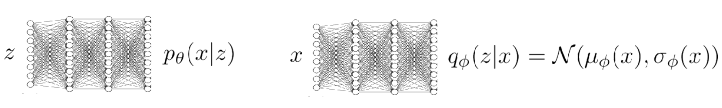
Instead of having a single per sample, we can train a network ! We will essentially obtain two networks. This model would output the necessary parameters and . This technique is called amortized variational inference.
In this case, we will obtain the new training process as follows:
- Sample mini-batch of .
- Calculate :
- Sample .
- ,
- .
- .
Now, we need to look more at $\nabla_\phi \mathcal{L} = \nabla_\phi \mathbb{E}_{z \sim q_\phi}\left[\log p_\theta(x_i \vert z) + \log p(z)\right] + \mathcal{H}(q_\phi(z))$. Let’s call $r(x_i, z) = \log p_\theta(x_i \vert z) + \log p(z)$. The question now becomes how do we calculate $\nabla_\phi \mathbb{E}_{z \sim q_i}\left[r(x_i, z)\right]$?
Unfortunately, this is non-differentiable, as it depends on samples from . Luckily there is a technique called the reparameterization trick for the normal distribution, which works as follows:
In the equation above, . We can now rewrite the gradient of the bottleneck as
Since is independent of , as you can see in the equations above, we can do backpropagation after applying this trick! However, we still need to sample in order to approximate the expectation. In practice, it seems that sampling once works well! This is likely the case because the normal distribution is quite centred around its mean, so one sample is often representative enough of an approximation.
The benefits to this methods are that, even though the proofs might be a bit non-trivial, it is very easy to implement. Furthermore, is has low variance. Unfortunately though, the reparameterization trick only works with continuous (normal) latent variables. However, there are papers that address this, such as vector-quantized variational autoencoders [7].
Practical examples
Variational autoencoders
We previous saw the following ELBO objective:
With some simply algebra, this can actually be rewritten into
In this case, for normal random variables, has a convenient analytical form! Using the reparameterization trick and by sampling one , the final objective can be written as
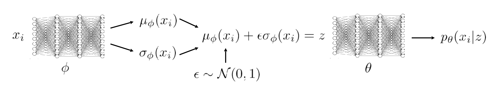
This can very conveniently be expressed with the networks in the figure above. There is an encoder model $q_\phi$ which takes an input $x_i$ and compresses it into a latent space $z$, where noise is added to the latent variable. The original input is then “reconstructed” from the latent variable using $p_\theta(x_i\vert z)$. At inference time, you can generate similar samples to your input simply by sampling multiple $\epsilon$ and reconstructing them! This can also be seen in the image on the right. This was introduced in [4].
Conditional models
The idea in [8] stays very similar to variational autoencoders. But now, we will try to model the conditional distribution instead of just . The loss stays almost identical, but we just condition on :
Now, can represent image data or whatever is necessary for conditional generation!
References
- Ruben Villegas, Mohammad Babaeizadeh, Pieter-Jan Kindermans, Hernan Moraldo, Han Zhang, Mohammad Taghi Saffar, Santiago Castro, Julius Kunze, Dumitru Erhan. Phenaki: Variable length video generation from open domain textual descriptions. International Conference on Learning Representations. 2022.
- Mark Woodward, Chelsea Finn. Active one-shot learning. arXiv preprint arXiv:1702.06559. 2017.
- Ian Goodfellow, Jean Pouget-Abadie, Mehdi Mirza, Bing Xu, David Warde-Farley, Sherjil Ozair, Aaron Courville, Yoshua Bengio. Generative adversarial networks. Communications of the ACM. 2020.
- Diederik P Kingma, Max Welling. Auto-encoding variational bayes. arXiv preprint arXiv:1312.6114. 2013.
- Ivan Kobyzev, Simon JD Prince, Marcus A Brubaker. Normalizing flows: An introduction and review of current methods. IEEE transactions on pattern analysis and machine intelligence. 2020.
- Jonathan Ho, Ajay Jain, Pieter Abbeel. Denoising diffusion probabilistic models. Advances in neural information processing systems. 2020.
- Aaron Van Den Oord, Oriol Vinyals, others. Neural discrete representation learning. Advances in neural information processing systems. 2017.
- Ali Razavi, Aaron Van den Oord, Oriol Vinyals. Generating diverse high-fidelity images with vq-vae-2. Advances in neural information processing systems. 2019.