CS-330 Lecture 5: Few-Shot Learning via Metric Learning
This lecture is part of the CS-330 Deep Multi-Task and Meta Learning course, taught by Chelsea Finn in Fall 2023 at Stanford. The goal of this lecture is to to understand the third form of meta learning: non-parametric few-shot learning. We will also compare the three different methods of meta learning. Finally, we give practical examples of meta learning, in domains such as imitation learning, drug discovery, motion prediction, and language generation!
Lars Quaedvlieg ·
The goal of this lecture is to understand the third form of meta learning: non-parametric few-shot learning. We will also compare the three different methods of meta learning. Finally, we give practical examples of meta learning, in domains such as imitation learning, drug discovery, motion prediction, and language generation! If you missed the previous lecture, which was about optimization-based meta learning, you can head over here to view it.
As always, since I am still new to this blogging thing, reach out to me if you have any feedback on my writing, the flow of information, or whatever! You can contact me through LinkedIn. ☺
The link to the lecture slides can be found here.
Quick recap
So far, we have discussed two approaches to meta learning: black-box meta learning, and optimization-based meta learning.
-
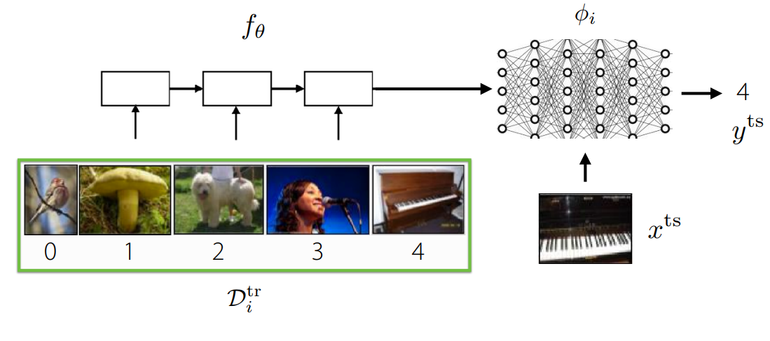
Computation pipeline for black-box meta learning. In black-box meta learning, we attempt to train some sort of meta-model to output task-specific parameters or contextual information, which can then be used by another model to solve that task. We saw that this method is very expressive (e.g. it can model many tasks). However, it also requires solving a challenging optimization problem, which is incredibly data-inefficient.
-
Optimization-based meta learning.
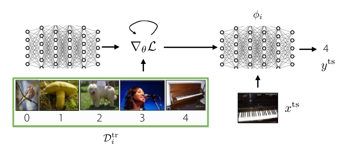
Computation pipeline for optimization-based meta learning. We then talked about optimization-based meta learning, which embeds an optimization process within the inner learning process. This way, you can learn to find parameters to a model such that optimizing these parameters to specific tasks is as effective and efficient as possible. We saw that model-agnostic meta learning preserves expressiveness over tasks, but it remains memory-intensive, and requires solving a second-order optimization problem.
Non-parametric few-shot learning
In the previous two approaches to meta learning, we only talked about parametric methods (A parametric model assumes a specific form for the underlying function between variables, using a finite number of parameters, while a non-parametric model makes fewer assumptions about the function form, potentially using an infinite number of parameters to model the data more flexibly.). However, what if we can avoid the optimization process in the inner learning loop of optimization-based meta learning methods? If this is possible, we do not have to solve a second-order optimization problem anymore. For this reason, we will look into replacing the parametric models in the inner learning loop with non-parametric models, which don’t require to be optimized. Specifically, we will try to use parametric meta learners that produce non-parametric learners.
One benefit of non-parametric methods is that they generally work well in low data regimes, making it a great opportunity for few-shot learning problems at meta-test time. Nevertheless, during meta-training time, we would still like to use a parametric learner to exploit the potentially large amounts of data.
The key idea behind non-parametric approaches is to compare the task-specific test data to the data in the train dataset. We will continue using the example of the few-shot image classification problem, as in the previous posts. If you want to compare images to each other, you need to come up with a certain metric to do so.
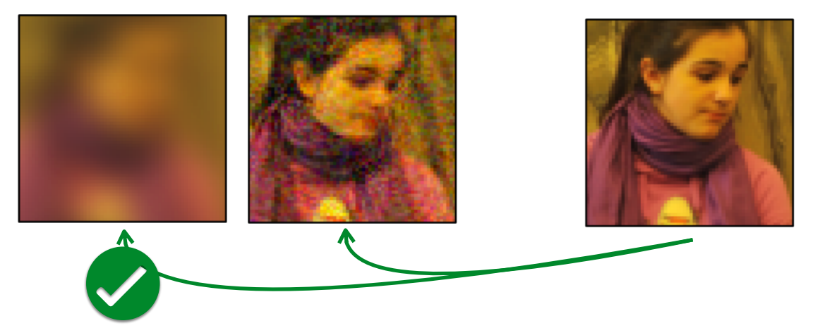
The simplest idea might be to utilize the -distance. Unfortunately, it is not that simple. If you look at the figure above, you can see the image of a woman on the right and two augmented versions on the left. When you calculate the -distance between the original image and the augmented image, the distance between the blurry image and the original one is smaller than the other distortion, even though this may resemble the original image more. For this problem, you could use a different metric, such as a perceptual loss function [1], but in general, it might be worthwhile to learn the metric from the data.
In this post, we will discuss three different ways of doing metric learning, starting with the easiest and building our way up. Firstly, we will talk about the most basic model: Siamese networks.
Siamese networks
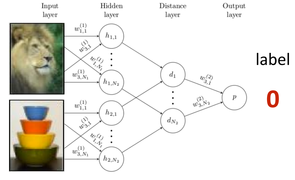
With a Siamese network, the goal is to learn whether two images belong to the same class or not. The input to the model is two images, and it outputs whether it thinks they belong to the same class. However, the penultimate activations correspond to a learned distance metric between these images. At meta-train time, you are simply trying to minimize the binary cross-entropy loss.
At meta-test time, you need to compare the test image against every image in the test-time training dataset , and then select the class of the image that has the highest probability. This corresponds to the equation below (for simplicity of the equation, we assume that only one sample will have ). Furthermore, corresponds to the indicator function.
With this method, there is a mismatch between meta-training and meta-testing. During meta-training, you are solving a binary classification problem, whilst during meta-testing, you are solving an -way classification problem. You cannot phrase meta-training in the same way, since the indicator function makes non-differentiable. We will try to resolve this by introducing matching networks.
Matching networks
In the previous equation above, we saw that at meta-test time, we use the class of the most similar training example as the estimate of the test sample. In order to get rid of the mismatch between meta-training and meta-testing, we can rephrase the meta-testing objective similarly to what we saw. Let’s say we instead modify the procedure to use a mix of class predictions as a class estimate. This would result in the equation below.
At meta-train time, we can now use the same objective, and backpropagate through the cross-entropy loss . This way, both meta-training and meta-testing are aligned with the same procedure. Our meta-training process would become:
- Sample task .
- Sample two images per class, giving .
-
Compute $\hat{y}^\mathrm{test} = \sum_{(x_k, y_k) \sim \mathcal{D}^\mathrm{tr}_i} f_\theta(x^\mathrm{test}, x_k)y_k$.
- Backpropagate the loss with respect to .
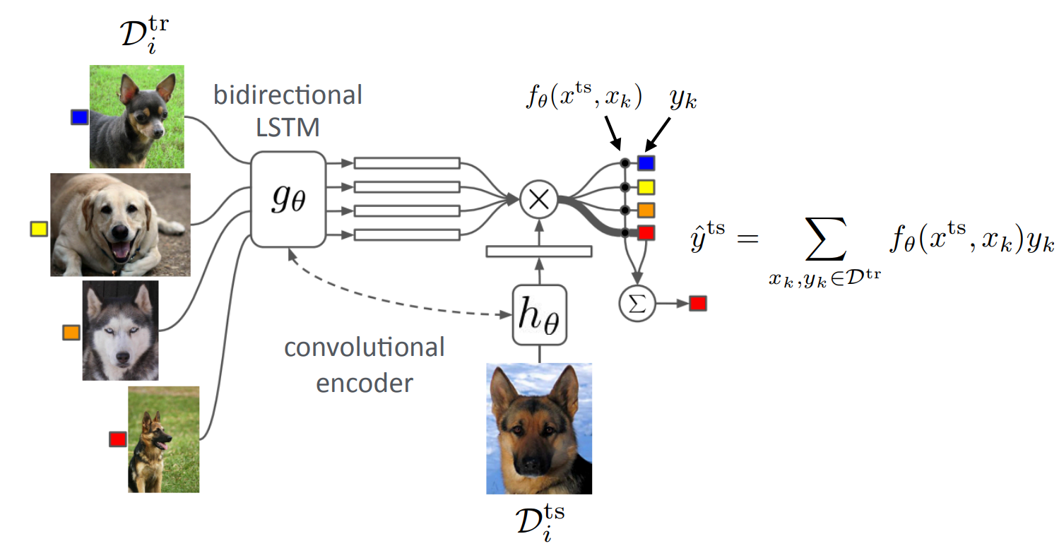
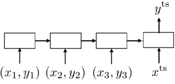
This idea corresponds to so-called “matching networks” [2]. Here, we embed each training image into some latent space using a bidirectional LSTM . Then, we encode the test image using a shared convolutional encoder and perform the dot product between the latent training vectors and the latent test vector, resulting in . Finally, we take the dot products with the labels to obtain the prediction This way meta-training and meta-testing match, which resulted in a better performance than something like Siamese networks.
Let’s stand still with what we’re doing for a second and think about how this approach is non-parametric. If we recall from parametric models, we would always compute task-specific parameters $\phi_i \leftarrow f_\theta(\mathcal{D}_i^\mathrm{tr})$. However, now have integrated the parameters $\phi$ out by computing $\hat{y}_j^\mathrm{test} := \sum_{(x_k, y_k) \sim \mathcal{D}^\mathrm{tr}} f_\theta(x_j^\mathrm{test}, x_k)y_k$ directly by comparing to the training dataset, making it non-parametric.

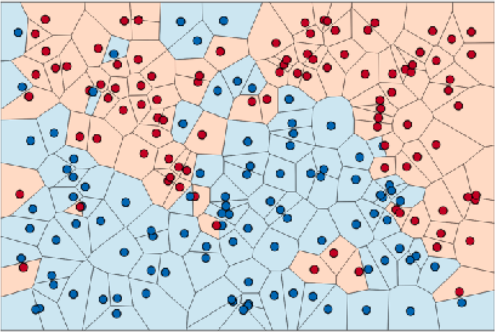
In the meta-training procedure described, we would sample two images per class. But what would happen if we sampled more than two images (ignoring potential class imbalance)? Well, with matching networks, each sample of each class is evaluated independently with $f_\theta(x_j^\mathrm{test}, x_k)$ instead of together. This could lead to strange results if the majority of a class has a low confidence but there is an outlier with a high confidence, overpowering the correct label. This can be depicted in the right figure. Imagine if you want to predict the label of the black square. The dot-product score with the red sample might be so high that it overpowers the other samples, even though it is more likely part of the blue class. We will try to resolve this by calculating prototypical embeddings that average class information.
Prototypical models
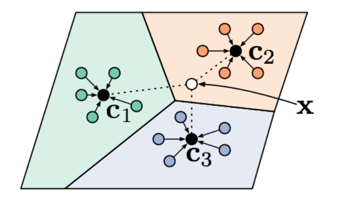
Prototypical models [3] will work quite similarly to what we have previously seen, but try to aggregate class information in order to prevent outliers. The figure on the right depicts this. Formally, we introduce class prototypes $c_n = \frac{1}{K} \sum_{(x,y)\in\mathcal{D}_i^\mathrm{tr}} 1(y_k=n)f_\theta(x_k)$. After we compute these class-averaged embeddings, a model will try to estimate the class of the test point by using something like Softmax probability, resulting in the equation below, where $d$ was the Euclidean or Cosine distance. Nevertheless, it could even be a learned network as we have previously seen.
As opposed to the matching networks, we are now using the same embedding function for both the training and testing datapoints.
More advanced models
The models that we talked about today are already quite expressive for non-parametric meta learning, but they all do some form of embedding followed by nearest-neighbours. However, sometimes you might need to reason about more complex relationships between datapoints. Let’s briefly discuss a few more recent works that approach this problem.
-
Relation networks [4].
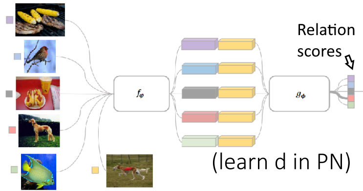
The idea is to learn non-linear relation modules on the embedding. They first embed the images and then compute this relation score, which corresponds to the distance function $d$ that we saw with prototypical models.
-
Infinite mixture of prototypes [5].
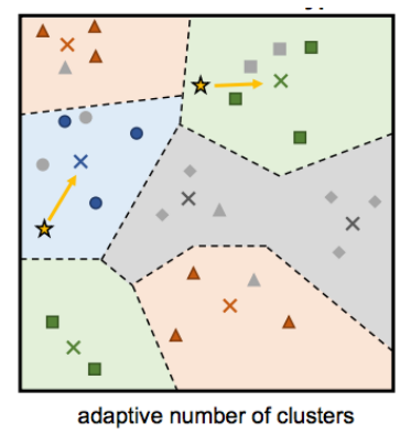
The idea is to learn an infinite mixture of prototypes, which is useful when classes are not easy to cluster nicely. For example, some breeds of cats might look similar to dogs, which would not be good when averaging class embeddings. In this case, we can have multiple prototypes per class.
-
Graph neural networks [6].
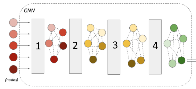
The idea is to do message passing on the embeddings instead of doing something as simple as nearest neighbours. This way, you can figure out relationships between different examples (i.e. by learning edge weights), and do more complex aggregation.
Properties of meta-learning algorithms
Now that we have seen all three different types of meta learning algorithms, we can compare each approach to see which problems might benefit from which approach. Let’s first quickly summarize all approaches.
Black-box meta learning.
<p>$y^\mathrm{ts} = f_\theta(\mathcal{D}_i^\mathrm{tr}, x^\mathrm{ts})$.</p>Optimization-based meta learning.
<p>$y^\mathrm{ts} = f_\mathrm{MAML}(\mathcal{D}_i^\mathrm{tr}, x^\mathrm{ts}) = f_{\phi_i}(x^\mathrm{ts})$, where $\phi_i = \theta - \alpha \nabla_\theta \mathcal{L}(\theta, \mathcal{D}^\mathrm{tr})$.</p>Non-parametric meta learning.
<p>$y^\mathrm{ts} = f_\mathrm{PN}(\mathcal{D}_i^\mathrm{tr}, x^\mathrm{ts}) = \mathrm{softmax}(-d(f_\theta(x^\mathrm{ts}), c_n))$, where $c_n = \frac{1}{K} \sum_{(x,y)\in\mathcal{D}_i^\mathrm{tr}} 1(y_k=n)f_\theta(x_k)$.</p>As you can see, all these methods share this perspective of a computational graph that we discussed in earlier posts. You can easily mix-and-match different components of these computation graphs. Below are some examples of paper that try this:
- Gradient descent on relation network embeddings.
- Both condition on data and run gradient descent [7].
- Model-agnostic meta learning, but initialize last layer as a prototype network during meta-training [8].
Let’s make a table of the benefits and downsides of each method that we have discussed up to this point in the series:
| Black-box | Optimization-based | Non-parametric |
|---|---|---|
| [+] Complete expressive power | [~] Expressive for very deep models (in a supervised learning setting) | [+] Expressive for most architectures |
| [-] Not consistent | [+] Consistent, reduces to gradient descent | [~] Consistent under certain conditions |
| [+] Easy to combine with a variety of learning problems | [+] Positive inductive bias at the start of meta learning, handles varying and large number of classes well | [+] Entirely feedforward, computationally fast and easy to optimize |
| [-] Challenging optimization problem (no inductive bias at initialization) | [-] Second-order optimization problem | [-] Harder to generalize for varying number of classes |
| [-] Often data-inefficient | [-] Compute- and memory-intensive | [-] So far limited to classification |
- Expressive power: The ability of to model a range of learning procedures.
- Consistency: Learned learning procedure will monotonically improve with more data
- Uncertainty awareness: Ability to reason about ambiguity during learning.
We have not yet discussed the uncertainty awareness of methods, but it plays an important role in active learning, calibrated uncertainty, reinforcement learning, and principled Bayes approaches. We will discuss this later on in the series!
Examples of meta learning in practice
In this section, we will very briefly talk about 6 different problem settings where meta learning has been used, some of which we have already seen in previous posts. This should give you a good idea of some different applications, and show you that it can be utilized in many different domains.
Land-cover classification
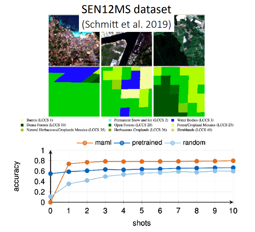
The goal of this paper [9] is to classify and segment satellite images in different regions of the world. Every region corresponds to a task, and the datasets are thus images from a particular region. The problem is that manually segmenting this data is expensive, so the authors use meta learning to quickly be able to segment new regions given limited training data on these regions.
Model: Optimization-based (model-agnostic meta learning)
Student feedback generation
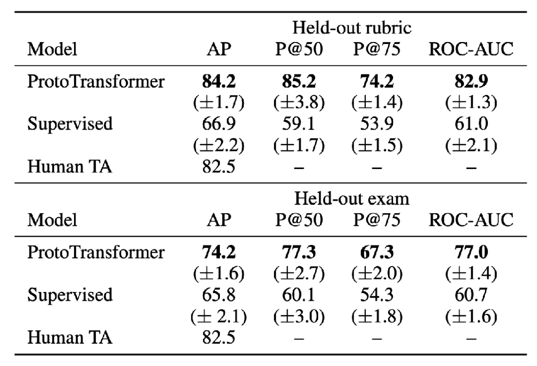

The goal of this paper [10] is to automatically provide students with feedback on coding assignments for high-quality Computer Science education. The different tasks corresponded to different rubrics for different assignments or exams. The datasets were then constructed of the solutions of the students (in this paper, they were always Python programs).
Supervised baseline: Train a classifier per task, using same pre-trained CodeBERT [11].
Outperforms supervised learning by 8-17%, and more accurate than human TA on held-out rubric! However, there is room for improvement on a held-out exam.
Model: Non-parametric (prototypical network with pre-trained Transformer, task information, and side information).
Low-resource molecular property prediction
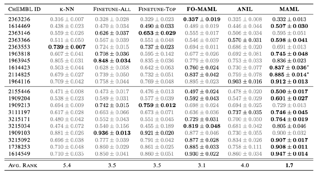
The goal of this paper [12] is to predict certain chemical properties and activities of different molecules in Silico models, which could potentially be useful for low-resolution drug discovery problems. The tasks here correspond to different chemical properties and activations, and the corresponding datasets are different instances of these properties and activations.
Model: Optimization-based MAML, first-order MAML, and an ANIL Gated graph neural net base model.
One-shot imitation learning
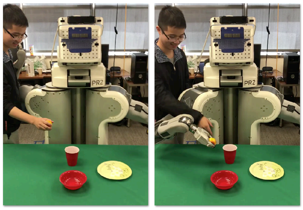
The goal of this paper [13] is to do one-shot imitation learning for object manipulation by using video demonstrations of a human. The tasks would be different manipulation problems. The training dataset would be the human demonstration, and the testing dataset would be the tele-operated demonstration.
Note: See that they training and testing datasets do not need to be sampled independently from the overall dataset for meta learning to work!
Model: Model-agnostic meta learning with learned inner loss function.
Dermatological image classification
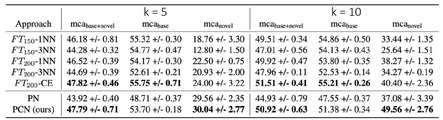
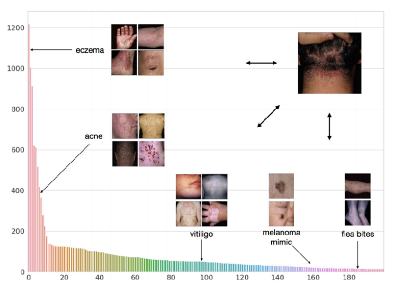
The goal of this paper [14] is to perform dermatological image classification that is good for all different skin conditions, which are the tasks in this case. The datasets consist of images of these skin conditions from different people.
Model: Non-parametric prototype networks with multiple prototypes per class using clustering objective.
Results show that the clustering prototype networks perform better than normal ones and competitive against a ResNet model that is pre-trained on ImageNet and fine-tuned on 200 classes with balancing. This is a very strong baseline with access to more info during training, and it requires re-training for new classes.
Few-shot human motion prediction
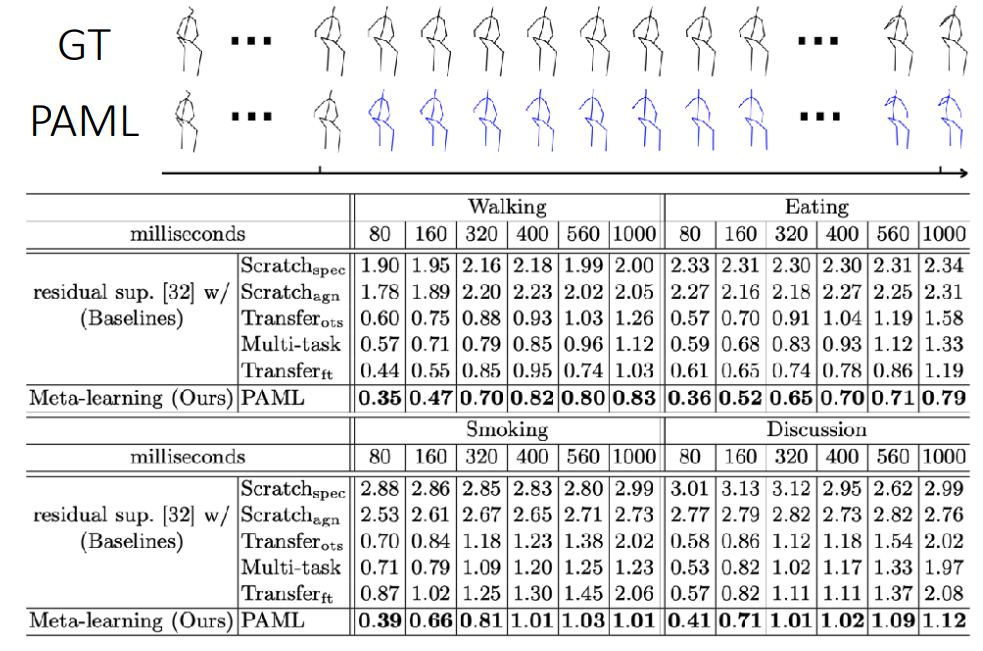
The goal of this paper [15] is to do few-shot motion prediction using meta learning, which could potentially be useful for autonomous driving and human-robot interaction. The tasks are different humans and different motivation. The corresponding train dataset $\mathcal{D}^\mathrm{tr}_i$ is composed of the past $K$ seconds of the motion, and the test set $\mathcal{D}^\mathrm{test}_i$ is composed of the future second(s) of the motion.
Note: See that they training and testing datasets do not need to be sampled independently from the overall dataset for meta learning to work!
Model: Optimization-based/black-box hybrid, MAML with additional learned update rule and a recurrent neural net base model.
References
- Justin Johnson, Alexandre Alahi, Li Fei-Fei. Perceptual losses for real-time style transfer and super-resolution. Computer Vision--ECCV 2016: 14th European Conference, Amsterdam, The Netherlands, October 11-14, 2016, Proceedings, Part II 14. 2016.
- Oriol Vinyals, Charles Blundell, Timothy Lillicrap, Daan Wierstra, others. Matching networks for one shot learning. Advances in neural information processing systems. 2016.
- Jake Snell, Kevin Swersky, Richard Zemel. Prototypical networks for few-shot learning. Advances in neural information processing systems. 2017.
- Flood Sung, Yongxin Yang, Li Zhang, Tao Xiang, Philip HS Torr, Timothy M Hospedales. Learning to compare: Relation network for few-shot learning. Proceedings of the IEEE conference on computer vision and pattern recognition. 2018.
- Kelsey Allen, Evan Shelhamer, Hanul Shin, Joshua Tenenbaum. Infinite mixture prototypes for few-shot learning. International conference on machine learning. 2019.
- Victor Garcia, Joan Bruna. Few-shot learning with graph neural networks. arXiv preprint arXiv:1711.04043. 2017.
- Andrei A Rusu, Dushyant Rao, Jakub Sygnowski, Oriol Vinyals, Razvan Pascanu, Simon Osindero, Raia Hadsell. Meta-learning with latent embedding optimization. arXiv preprint arXiv:1807.05960. 2018.
- Eleni Triantafillou, Tyler Zhu, Vincent Dumoulin, Pascal Lamblin, Utku Evci, Kelvin Xu, Ross Goroshin, Carles Gelada, Kevin Swersky, Pierre-Antoine Manzagol, others. Meta-dataset: A dataset of datasets for learning to learn from few examples. arXiv preprint arXiv:1903.03096. 2019.
- Marc Ru\sswurm, Sherrie Wang, Marco Korner, David Lobell. Meta-learning for few-shot land cover classification. Proceedings of the ieee/cvf conference on computer vision and pattern recognition workshops. 2020.
- Mike Wu, Noah Goodman, Chris Piech, Chelsea Finn. Prototransformer: A meta-learning approach to providing student feedback. arXiv preprint arXiv:2107.14035. 2021.
- Zhangyin Feng, Daya Guo, Duyu Tang, Nan Duan, Xiaocheng Feng, Ming Gong, Linjun Shou, Bing Qin, Ting Liu, Daxin Jiang, others. Codebert: A pre-trained model for programming and natural languages. arXiv preprint arXiv:2002.08155. 2020.
- Cuong Q Nguyen, Constantine Kreatsoulas, Kim M Branson. Meta-learning GNN initializations for low-resource molecular property prediction. arXiv preprint arXiv:2003.05996. 2020.
- Tianhe Yu, Chelsea Finn, Annie Xie, Sudeep Dasari, Tianhao Zhang, Pieter Abbeel, Sergey Levine. One-shot imitation from observing humans via domain-adaptive meta-learning. arXiv preprint arXiv:1802.01557. 2018.
- Viraj Prabhu, Anitha Kannan, Murali Ravuri, Manish Chablani, David Sontag, Xavier Amatriain. Prototypical Clustering Networks for Dermatological Image Classification.
- Liang-Yan Gui, Yu-Xiong Wang, Deva Ramanan, Jos\'e MF Moura. Few-shot human motion prediction via meta-learning. Proceedings of the European Conference on Computer Vision (ECCV). 2018.