CS-330 Lecture 7: Unsupervised Pre-Training: Reconstruction-Based Methods

This lecture is part of the CS-330 Deep Multi-Task and Meta Learning course, taught by Chelsea Finn in Fall 2023 at Stanford. The goal of this post is to introduce to widely-used methods for unsupervised pre-training, which is essential in many fields nowadays, most notably in the development of foundation models. We also introduce methods that help with efficient fine-tuning of pre-trained models!

The goal of this post is to introduce to widely-used methods for unsupervised pre-training, which is essential in many fields nowadays, most notably in the development of foundation models. We also introduce methods that help with efficient fine-tuning of pre-trained models! If you missed the previous post, which was about unsupervised pre-training with contrastive learning, you can head over here to view it.

As always, since I am still quite new to this blogging thing, reach out to me if you have any feedback on my writing, the flow of information, or whatever! You can contact me through LinkedIn. ☺

The link to the lecture slides can be found here.

Note: The lecture that I have based this post on is probably one of my favourite ones so far. Although we might not discuss the full details of every method, we will introduce a ton of cool things, and I am confident that you can learn a lot from it! In any case, I always reference corresponding papers, so feel free to check those out in addition to this blogpost!

Quick recap and introduction

Alt text. — The process of doing unsupervised pre-training for few-shot learning.

In the previous post, we introduced the idea of unsupervised pre-training for few-shot learning, as we also highlight in the figure above. Given an unlabelled dataset ${x_i}$, we do some form of unsupervised pre-training to learn a representation of the data. This way, it is easy to fine-tune the model on task-specific problems when we have labelled (for the sake of simplicity) samples.

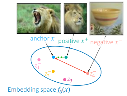
We already talked about contrastive learning, which comes from the idea that similar (positive) samples in a dataset should have similar representations, and differing (negative) ones should be different! After improving different approaches for a while, we introduced SimCLR, which tries to learn these representations by sampling a positive and many negative examples, somehow derived from the original dataset. This is also shown (on a very high level) in the figure on the right.

Unfortunately, the main drawback of this method was the large batch size or training time that is required to produce good models, which makes it less favourable for huge unsupervised datasets. We also talked about some newer methods that try to address these issues, but in this post, we will talk about another way to pre-train a model on unsupervised data: reconstruction-based methods. As you will see, one advantage of this method is that representations can be learned without explicitly comparing different samples to each other.

The intuition behind reconstruction-based methods comes from the idea that a good representation of a sample should be sufficient to reconstruct it. In contrast with contrastive learning, this means that we do not need to work about things like sampling enough difficult negative samples and having large batch sizes.

Autoencoders

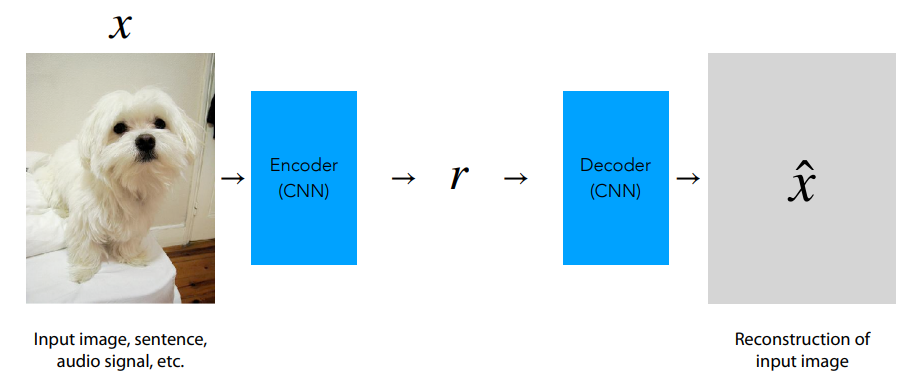
Let’s immediately try to think about what a reconstruction-based model could look like. Let’s say we have a model $\hat{x} =f_\theta(x)$, that tries to reconstruct its input. We split the model into two parts:

The encoder, which is responsible for projecting the input, in this case an image, into an embedding $r$.
The decoder, which takes the input embedding $r$ and attempts to reconstruct the original sample $x$ from it. Its output is $\hat{x}$.

If the encoder produces a “good” representation of the input with $r$, meaning that $r$ contains enough information to reconstruct $x$, then a reasonably-sized decoder should be able to produce a reconstruction $\hat{x}$ that is very close to the input $x$ in some metric space. As a simple loss function, we can then consider a distance measure, such as the $\ell_2$-distance $d(x, \hat{x}) = \Vert x - \hat{x} \Vert^2$.

However, try to think about what happens if $r$ can be anything. Is this a good idea?

Toggle answer.

Answer: No! It might be obvious, but if $r$ can be anything, then we can let $r = x$. In this case, one optimal solution to the encoder and decoder would be to just let $\theta$ be the identity function, since the reconstruction will be perfect.

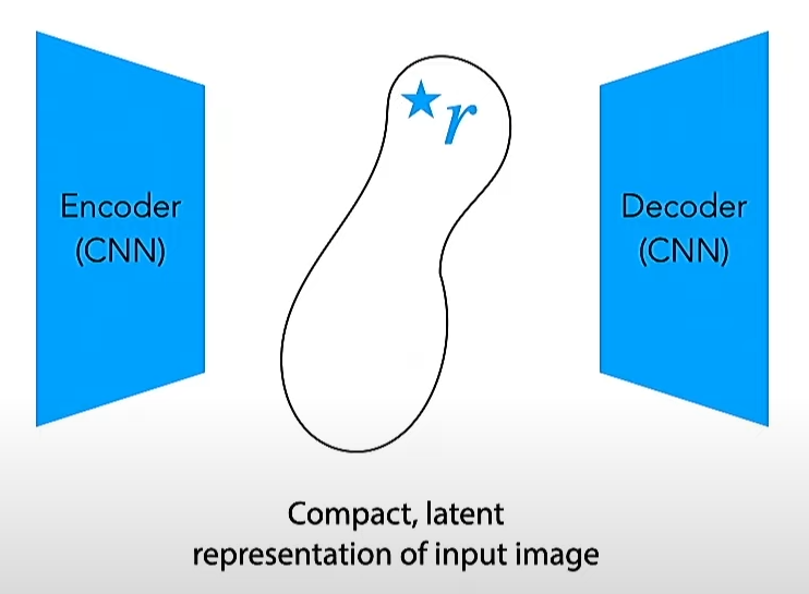
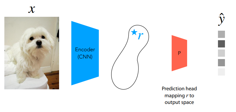
Instead, we need to ensure that $r$, the encoder output, is a useful, lower-dimensional representation of the input sample $x$. This is done very easily by letting the encoder project the input onto a compact latent representation With latent representation, we mean that the representation $r$ is an unobserved statistic (e.g. we do not directly observe it) of the input image. The hope is then that the latent dimensions are forced to represent high-level concepts that generalize to other tasks by filtering out sample-specific noise and keeping track of the useful structure between samples.

In order to do few-shot learning on a trained autoencoder, we only need the encoder. We first project out input sample into the compact latent variable $r$. Then, we can simply add a prediction head that takes this input and maps it to the necessary task-specific output space. This is identical to how we use the representations that we saw in the contrastive learning post. Usually, the encoder is frozen (i.e. its weights are not updated during fine-tuning), and only the prediction head is fine-tuned on the few-shot data.

This approach is very simply and expressive, the only choice that we have is the distance metric $d(x, \hat{x})$, and there is no need to select positive and negative pairs! However, we need to design some way to bottleneck the model, and in practice, the model generally does not give very good few-shot performance.

This lack of few-shot performance mainly comes from the fact that high-level generalizable features are still not really obtained, even when training a compact model. In reality, the models often just try to learn a hash of $x$ rather than a conceptual summary, so the reconstruction loss is still low but it is not useful for few-shot fine-tuning.

There are many existing strategies that try to approach this issue. They encourage the encoder to extract high-level features in the following ways:

Information bottlenecks: Adding noise to force the model to learn features invariant to the noise.
Sparsity bottlenecks: The representation should have zeros in most dimensions, to encourage dimensions to contain useful information.
Capacity bottlenecks: The decoder is limited in capabilities so that the encoder is forced to create useful representations.

Masked autoencoders

Whilst a lot of research has gone, and is still going into designing different bottlenecks, we nowadays stop worrying about designing these bottlenecks and make the problem more difficult to solve. However, if the model is able to solve this problem, we are sure that it must have learned a useful representation of the data.

This harder problem is addressed by a class of models that are referred to as “masked autoencoder”. This term encompasses many of the foundation models that are used in practice nowadays. In this post, we fill focus on two fundamental models: BERT and MAE, but there are many other models that exist nowadays.

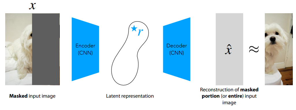
Let’s first talk about this “harder problem”. With regular autoencoders, we bottleneck $r$ to avoid totally degenerate solutions (i.e. convergence to the identity function). But what if the task is just “too easy”, and it only admits to unhelpful solutions? In this case, we can try to mask a part of the input (and/or output) sample, in order to encourage the model to learn more meaningful features. This solves a more difficult learning task, since the model now has to reconstruct the masked part of the sample with less to no information about it. The general recipe for pre-training masked autoencoders is as follows:

Choose a distance metric $d(\cdot, \cdot) \rightarrow \mathbb{R}$ as a loss function.
Sample $\tilde{x}_i, y_i \sim \mathrm{mask}(x_i)$, where $\tilde{x}_i, y_i$ are two disjoint sub-regions of $x_i$ (or instead, sometimes, $y_i = x_i$).
Make prediction $\hat{y}_i = f_\theta(\tilde{x}_i)$.
Compute the loss $\mathcal{L}_i= d(y_i, \hat{y}_i)$.

You might wonder how we parameterize $f_\theta$ in this case? While this can depend on the problem, in practice, Transformers are nowadays almost exclusively used!

Bidirectional Encoder Representations from Transformers (BERT)

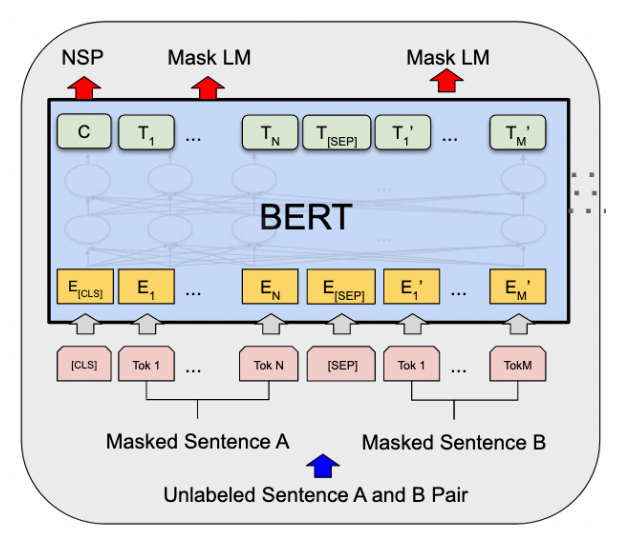
BERT is probably the most famous example of a masked autoencoder for language. It takes a string, which can be multiple sentences as input, and randomly replaces words within this string with special <mask>. The goal of the model is then to reconstruct the masked words given the context, which is the rest of the unmasked sentence. The model itself consists of a bidirectional Transformer, meaning that the mask tokens can attend to any other token in the sequence I am using the term token here. A token represents the smallest unit of data that you are using, such as a word in text, a pixel (or image patch) in images, or a frame in videos, allowing the a Transformer to process different types of input uniformly.. Tokenization facilitates the model's understanding and generation of complex, multimodal outputs by analysing patterns across varied data forms.). This is very important, since it means that this method is not autoregressive (e.g. it can look into the “future” of a sentence.

The following is an example of how BERT training works with a given input sentence:

Given the input sentence $x$, we create the masked sentence $\tilde{x}$ that masks the word tokens $y_2, y_6$, and $y_9$ (Biden, president, and was, respectively).
We then use the BERT model to produce $\hat{y} = p_\theta(\tilde{x})$. So, for all tokens in the input sentence $\tilde{x}$, BERT outputs a probability distribution.
Finally, we use the probabilities over the masked input tokens to compute the loss. In this case, we use KL-divergence as a loss function (this can be replaced though by other losses as well though). The loss becomes
\[d(y, \hat{y})=\sum_j \mathrm{KL}(y_j \Vert \hat{y}_j) = - \sum_{i \in \{2, 6, 9\}} \log(p_\theta(y_i \vert \tilde{x}))\;.\]

There are also some decisions that BERT makes on the masking. At any time, it selects $15$% tokens from the inputs. Then, $80$% of the time, the input is replaced by a masking token. The other $20$% of the time, the input token is instead replaced by a completely random token. However, this can also still be improved, by for example masking longer spans of text or selecting information-dense spans of text. The specific masking procedure can be vital for good generalization capabilities of the model!

Masked autoencoders for vision (MAE)

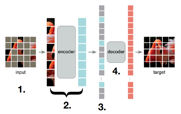
For vision, a similar model called MAE exists. It is essentially BERT for vision. It starts by splitting an input image $x$ into multiple patches, which is commonly done to tokenise images before putting them into a transformer. Every patch represents a token. Then, tokens (patches) are randomly masked, just as in BERT, and fed to an encoder. The decoder must then reconstruct the masked patches in the image. There are a few differences with BERT:

Instead of words, we have a sequence of image patches.
We mask ~$75$% of image patches.
We compute representations of only the unmasked patches.
We insert placeholder patches at the masked locations.
We decode the encoded representation back into the original image.

We can fine-tune this model by using the encoded representation of step 2 in the figure above.

It is very cool to see that MAEs give state-of-the-art few-shot image classification performance among models that are trained using unsupervised pre-training.

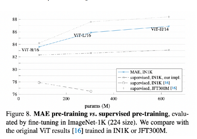
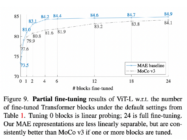
From the figures above you can observe the following: The unsupervised masked autoencoding recipe works better than pre-training with labels on the same data! Moreover, when fine-tuning the full model (not just linear probing Linear problem is a term that described adding just one linear head on top of the existing model. on frozen pretrained model), it performs better than (momentum-based) contrastive learning!

Transformers and efficient fine-tuning

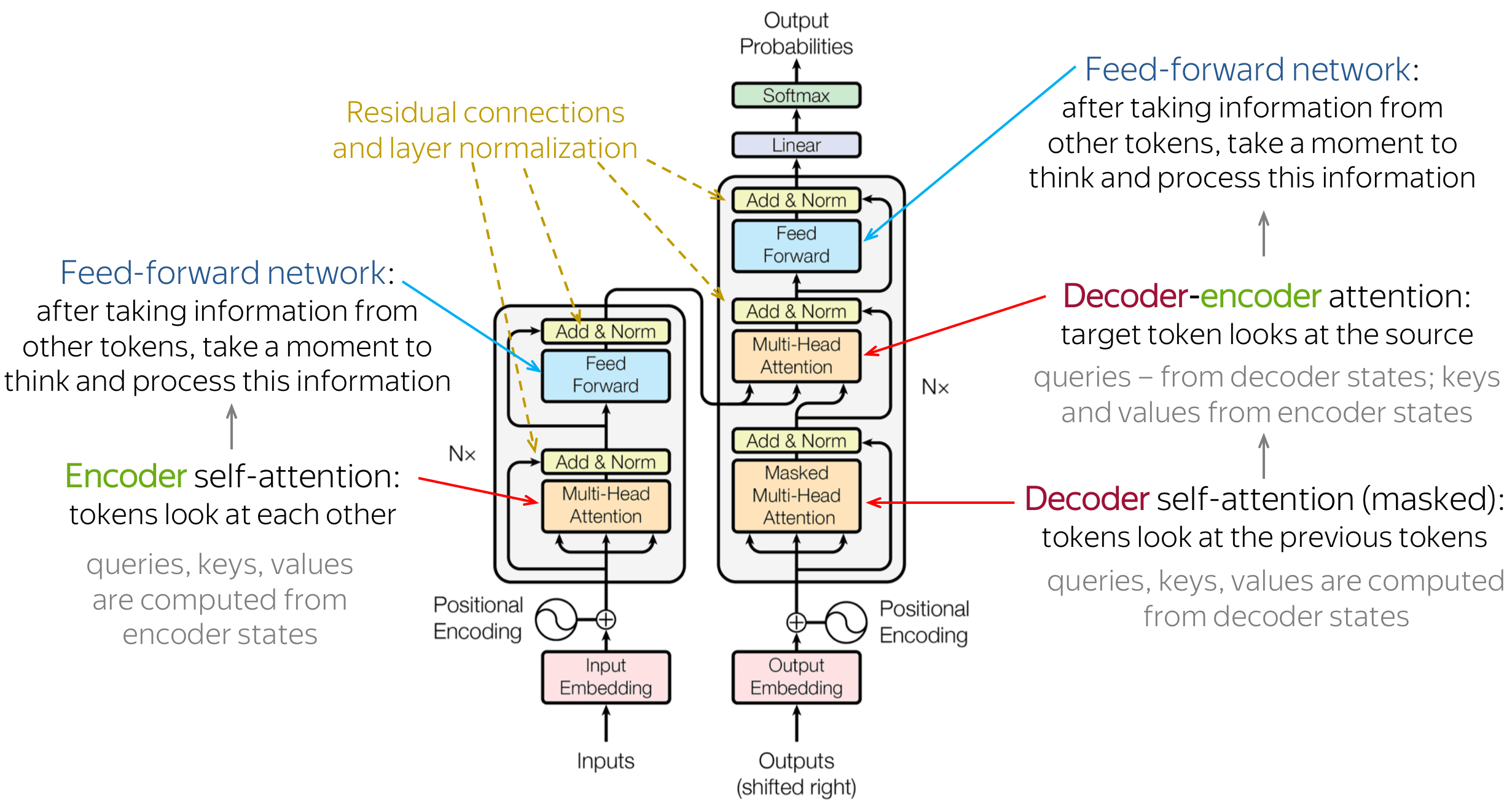
We have now seem a glimpse of what Transformer models can achieve together with a masked autoencoder scheme! If you are unfamiliar with Transformers, we will give a quick overview of the architecture. If you already know about Transformers, you might want to stick around when we talk about efficient fine-tuning later on!

For a detailed look into Transformers, I can recommend reading the “The Illustrated Transformer” blog. However, let’s quickly discuss the encoder architecture from the figure above step-by-step (please ignore the decoder in the figure):

Initially, we have inputs, which are quantified as tokens. Some examples of tokens:
- Text: Tokens could be words
- Images: Tokens could be patches.
- Reinforcement Learning: Tokens could represents the states, actions, rewards, and terminal indicators.
We then put these tokens through their corresponding embedding layers. These layers are modality-specific. This means that if we have image tokens, we probably want to embed them differently (i.e. by using a VQ-VAE or a CNN) than with text tokens (with a lookup table).
Since the attention mechanism that we will explain is permutation invariant, meaning that its output does not depend on an order of tokens, we will need to add some positional encoding to it for sequence-based problems such as language. Do check out The Illustrated Transformer to learn more about positional encodings.
We now pass the embedded tokens with positional embeddings through a multi-head self-attention mechanism. This mechanism makes tokens “look at each other” to determine how much attention to pay to the other tokens. Let’s get into the formula of self-attention:
\[\mathrm{Attention}(Q, K, V) = \mathrm{softmax}(\frac{QK^T}{\sqrt{d}})V\;.\]
Here, $Q = XW^Q \in \mathbb{R}^{L \times d}$ are the query vectors, where $L$ is the number of tokens in the sequence and $d$ is the hidden size of the model. Moreover, $K = XW^K \in \mathbb{R}^{L \times d}$ are the key vectors, and finally, $V = XW^V \in \mathbb{R}^{L \times d}$ represent the values. We also have that $W^Q, W^K, W^V$ are the learnable weights. In this example, we let the hidden sizes be equal, but this does not necessarily have to be true.

Let’s go through this formula step-by-step. The intuition is as follows:
1. We first compute $Q$, $K$, and $V$. These are projections of the input $X$. The query semantically represents the elements we want to draw comparisons against, the key corresponds to elements we compare the query to, and the value represents the content that we actually want to retrieve or focus on based on these comparisons. Essentially, the mechanism computes the relevance of each key to a given query to determine how much attention to pay to each “value”, enabling the model to dynamically focus on important parts of the input data.
2. We then compute $\mathrm{softmax}(\frac{QK^T}{\sqrt{d}}) \in \mathbb{R}^{L \times L}$. For every token in the row, it essentially computes a softmax-distribution over all the other the other tokens. This can be interpreted as the “amount” of attention to pay to that other token.
3. Finally, we multiply the previous output by $V$, letting the result be of shape $\mathbb{R}^{L\times d}$. This multiplied the probability to pay attention to each tokens to that token’s corresponding value, creating a weighted sum of values. This represents the output of the self-attention, and the new embedding of the tokens!
Now that we have the new token embeddings from self-attention, we do layer normalization and put them through a fully-connected layer. At this point, you could do something like average or max pooling over all tokens and attach a head to the resulting vector. You can then fine-tune that head for few-shot learning on that representation!

I hope this short overview of the encoder in Transformers was at least a bit helpful! I know it can be a lot if you haven’t seen it before, so if you’re struggling that’s completely understandable! In that case, I recommend you to check out more comprehensive and intuitive blogposts.

For autoregressive generation in a Transformer decoder, you can also something very similar. The “main” difference is to do mask future tokens in the attention so that your attention mechanism isn’t look at future tokens. You can easily do this by manually setting the attention score before doing the softmax operation to $-\infty$ for those future tokens.

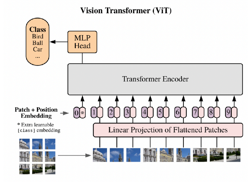
This idea can easily be extended to image-based tokens, which was introduced in the Vision Transformer (ViT) paper There are some subtle differences with the original Transformer, especially in the encoding and positional embeddings, but the idea stays the same:

Tokenize and embed your input.
Feed it through a Transformer encoder to get a representation for each token.
Perform pooling or something similar to get a vector representation. It is also possible to prepend a special token (i.e. [CLS] in BERT) to use as a final vector representation. The model should learn to put the useful information into the embedding of that special token.
Put a head on that final representation to perform fine-tuning for few-shot learning!

Low-rank adaptation of language models (LoRA)

Now that we know how to set up the Transformer encoder, we should ask ourselves how to fine-tune a pre-trained model. There are so many possible options, which are critical to the performance of our final model:

Freeze the pre-trained backbone.
Fine-tune everything.
Fine-tune some parameters?
Freeze the pre-trained backbone and inject new parameters?

In this section, we will focus on LoRA , which is very commonly used in practice to this day (March 2024). The key idea is that we wish to fine-tune our model just a little bit, so that we do not get rid of the useful knowledge that our pre-trained model has. For Large Language Models (LLMs), we also want to avoid the need to store a new version of every single parameter in the model.

In order to get an intuition of this idea, we go back to the associative memory view of the linear transformation. The linear transformation $W$ can be decomposed into $W = \sum_r v_ru_r^T$ for an r-rank matrix $W$ (with orthogonal $u_r$ by singular value decomposition). For this reason, we show the following:

\[Wx = \left(\sum_r v_ru_r^T\right)x = \sum_r v_r(u_r^T x)\;.\]

From this decomposition, it can be interpreted that $Wx$ produces a sum over memories in $v_r$, which are weighted by the memory relevance $u_r^T x$. Here, each $u_r^T$ is a key.

If we wish to only change the model a little bit, as we previously described, we can try to only make a low-rank change to $W$. With LoRA, you compute the new weights as follows:

\[W_\mathrm{ft} = W_0 + AB^T\;.\]

Here, $W_\mathrm{ft} \in \mathbb{R}^{d \times d}$ are the fine-tuned parameters, $W_0 \in \mathbb{R}^{d \times d}$ are the initial parameters, and $AB^T$ is a new low-rank residual (fine-tuned). Note that $A,B \in \mathbb{R}^{d \times p}$. It should thus be added to the old parameters. In practice, you initialize both $AB^T$ to zeros, since it is easier to fine-tune the model from the point where the model weights are $W_\mathrm{ft} = W_0 + 0 = W_0\;.$ Since you do not get any gradient if you set $A=B=0$, you can initialize only one to zeros and the other randomly.

With LoRA, you only need to store $2\cdot d\cdot p$ new parameters instead of the $2\cdot d^2$ of a completely new model.

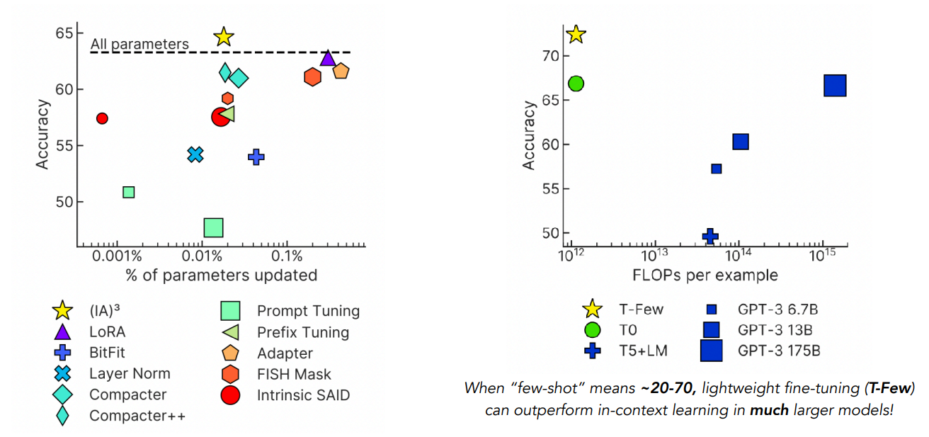
There are many more ways of “lightweight” fine-tuning models, which are evaluated in the T-Few paper . If you are interested, I encourage you to go through it! They also show that lightweight fine-tuning can be better for few-shot learning than in-context learning with models of $10$ to $100$ times bigger on the experiments that they performed!

Autoregressive models

There are some downsides to masked autoencoders. For example, you need to pick the mask to apply to the inputs, you are only using ~$15$% of the examples for training, and it is difficult to sample from.

The idea of autoregressive models is very simple. What if we just predict the next token? This way, you do not need to select a specific masking strategy, but you rather mask tokens that are in the future of a newly processed token. We show an example of this masking (denoted by the $-$) in the figure above. On the right side in this figure, you can see the model $p_\theta(x_t\vert x_{<t})$ that tries to predict the next token given the past ones.

Note that autoregressive models are just masked autoencoders with a specific masking function. There is also research that has been done into different masking schemes, with this paper being my favourite yet. They basically improve the memory capabilities of LLMs by including pause tokens.

These models form the basis for almost every single foundation model that is currently out there. We will briefly look into a case study for a multimodal autoregressive model called Flamingo.

Flamingo

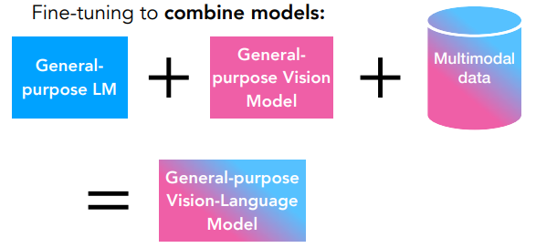
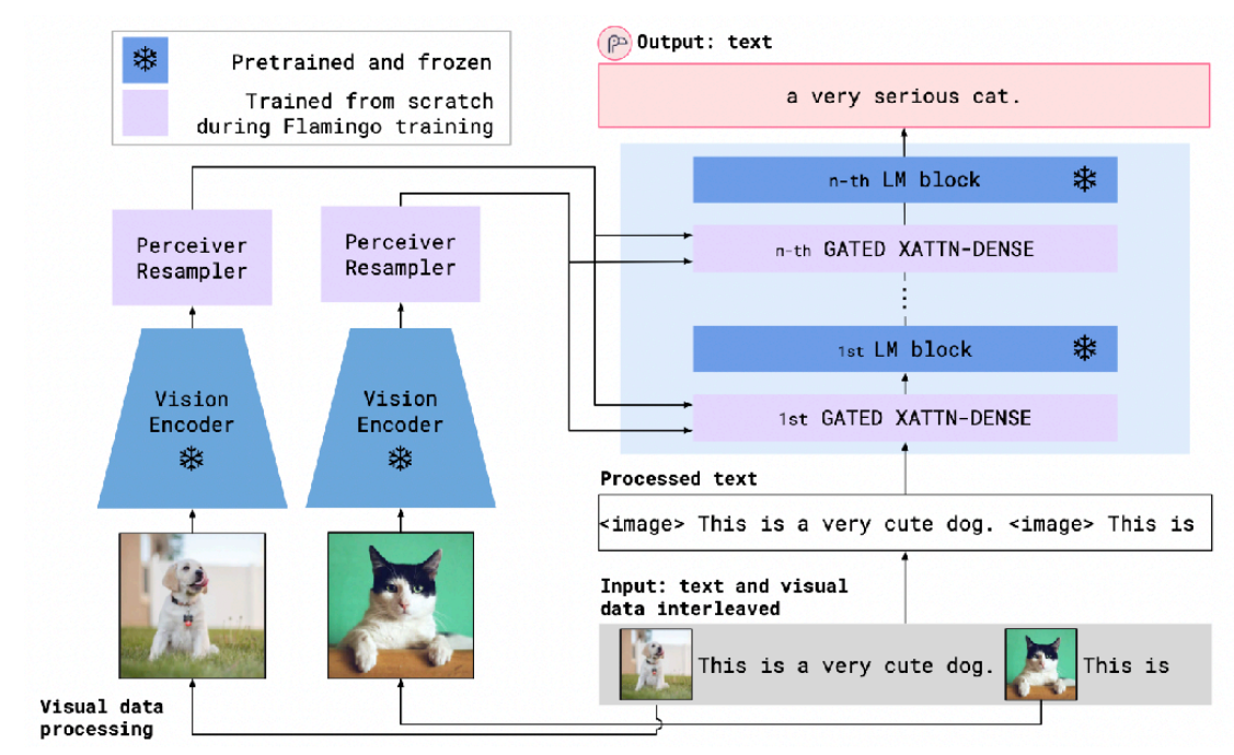
This paper shows that building a multimodal autoregressive model from scratch is a bad idea. Instead, they propose the idea of fine-tuning pre-trained models together with multimodal data to combine these models into a multimodal model.

The model architecture processes interleaved visual and textual data using a series of Vision Encoders, Perceiver Resamplers, GATED XATTN-DENSE blocks, and LM blocks to produce text output. The Vision Encoders, which are pretrained and frozen, transform images into a compatible representation, while the Perceiver Resamplers turns this spatiotemporal representation into a fixed-sized set of visual tokens. The model then integrates this visual information with text-based inputs using the GATED XATTN-DENSE blocks that enable cross-modality attention and interaction, complemented by LM blocks tailored for text understanding. This architecture allows Flamingo to generate text outputs that reflect a combined understanding of both the visual context provided by images and the semantics of the accompanying text.

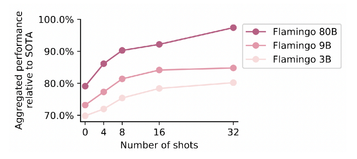
The cool thing is that you can now do in-context few-shot learning on sequences that freely mix text and images! This enables few-shot captioning, visual question-answering, etc. They also show that few-shot Flamingo performs approximately as well as non-few-shot state-of-the-art models (fine-tuned on the whole training set)!