CS-330 Lecture 6: Unsupervised Pre-Training: Contrastive Learning

This lecture is part of the CS-330 Deep Multi-Task and Meta Learning course, taught by Chelsea Finn in Fall 2023 at Stanford. The goal of this lecture is to understand the intuition, design choices, and implementation of contrastive learning for unsupervised representation learning. We will also talk about the relationship between contrastive learning and meta learning!

The goal of this lecture is to understand the intuition, design choices, and implementation of contrastive learning for unsupervised representation learning. We will also talk about the relationship between contrastive learning and meta learning! If you missed the previous lecture, which was about non-parametric few-shot learning, you can head over here to view it.

As always, since I am still quite new to this blogging thing, reach out to me if you have any feedback on my writing, the flow of information, or whatever! You can contact me through LinkedIn. ☺

The link to the lecture slides can be found here.

Quick introduction

Alt text. — Example of the amount of data needed for transfer learning through fine-tuning.

So far we have talked about the idea of few-shot learning via meta learning. In this problem, you are given a set of tasks $\mathcal{T}_1, \cdots, \mathcal{T}_n$ to train on, and wish to solve a new task $\mathcal{T}_\mathrm{test}$ more quickly, effectively, and stably. Before starting with meta learning, we discussed the idea of using transfer learning via fine-tuning for this problem, but the performance of this method is very dependent on the amount of data, as you can see on in figure above. Instead, we proposed three different types of meta learning to help quickly adapt to new tasks: black-box meta learning, optimization-based meta learning, and non-parametric meta learning.

These methods were shown to work especially well when there are many tasks available for a problem. But, when you only have few tasks, meta learning might not be a good approach to the problem due to risks of overfitting and having insufficient diversity in your data. Let’s take this even further. What if you only have one batch of unlabelled data?

In this case, meta learning might not be a good approach to the problem. Instead, we will look into unsupervised representation learning for few-shot learning. In the figure above, we describe the process of training a model for this problem on a high level. Given a dataset of unlabelled data ${x_i}$, we want to do unsupervised pre-training to get an initial model. Once we have obtained this model, we then wish to fine-tune it on a task-specific dataset $\mathcal{D}_j^\mathrm{tr}$, to get a task-specific predictor.

You might have already noticed that this procedure is very similar to the way that large language models are trained. They are first pre-trained on a huge corpus of language data, and then fine-tuned for specific purposes (i.e. alignment, mathematics, etc.).

In this course, we will talk about two approaches to this problem:

Contrastive learning.
Reconstruction-based methods.

In this post, we will focus on contrastive learning, and we will discuss the reconstruction-based methods in the next one!

Contrastive learning

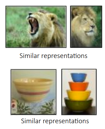
The idea behind contrastive learning is that similar examples should have similar representations, and different examples should have different representations. When you have a batch of unsupervised data, you can decide on a semantic meaning of similarity and then learn the data representations as embeddings from a model. The steps would roughly be as follows:

Select or generate examples that are semantically similar.
Train an encoder where similar examples are closer in the representation space than non-similar examples.

Let’s start out with a simple approach. We are trying to learn an model $f_\theta(x)$, which embeds a datapoint $x$ into some representation. As a loss function, we decide use the following:

\[\min_\theta \sum_{(x_i, x_j)}\Vert f_\theta(x_i) - f_\theta(x_j)\Vert^2\;.\]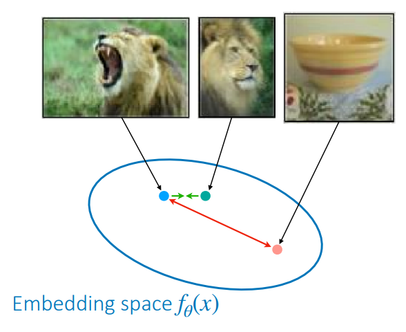

This loss function tries to minimize the distance of the embeddings of similar datapoints $x_i$ and $x_j$. However, do you think this loss function performs well? Well, you might be able to see that one possible optimal solution to this loss function would just be to let $f_\theta(x) = 0$. This would mean that all datapoints are mapped to the same representation, even very different datapoints. For this reason, the loss should also incorporate an element to push apart differing samples. You need to both compare and contrast!

We present this idea in the figure on the right. In the embedding space, similar samples should be close, whilst differing samples should should be far apart. The key design choices here are choosing what to compare/contrast, and which contrastive loss you use.

Whilst the ideas work for all kinds of unlabelled data, we will focus on images (or videos) in the remainder of this post. Recalling that similar examples should have similar representations, we discuss a few ways to measure similarity in images.

The most straightforward way to assign similarity is by looking at class labels. This is very related to the Siamese networks and Prototypical networks that we saw in the previous post. However, for unsupervised data, this is not possible. Instead, there are many different approaches that create new samples from one sample. Below are some examples .

Patch-based.

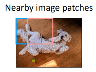
Given an image, it is possible to split it into image patches, and to let image patches that are close to each other have a similar representation.

Augmentation-based.

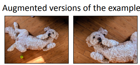
Given an image, it is also possible to augment it in some way (i.e. by flipping, cropping, etc.), and letting those sample be similar to each other.

Temporally-based.

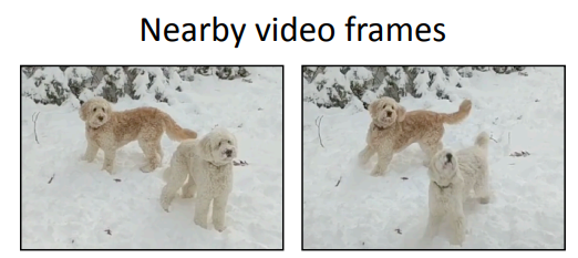
Given a video, it is often possible to let frames that are temporally close have a similar representation. Of course this depends on the nature of the video.

As you can see, defining similarity is usually pretty problem-specific. A simple example in text would be something like bag of words depending on the task, or permutations with a similar semantic meaning.

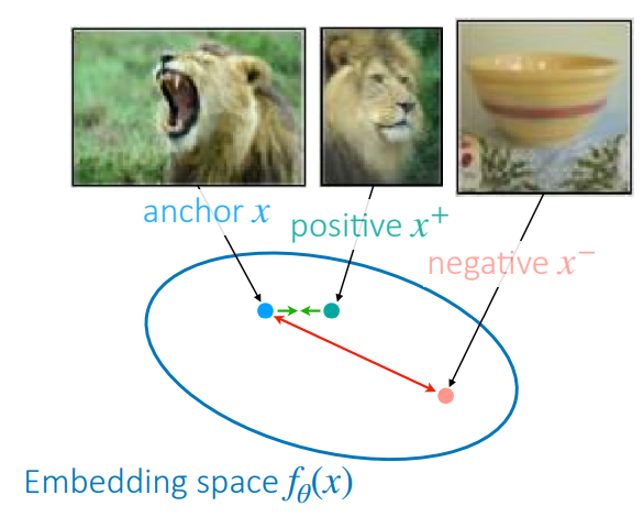
Now that we have a way of defining similarity across samples, we can take a look at modifying the loss function to push apart differing samples. One common loss function is the triplet loss, introduced in , which simply tries to push away unrelated samples:

\[\min_\theta \sum_{(x, x^+, x^-)}\max(0,\Vert f_\theta(x) - f_\theta(x^+)\Vert^2 - \Vert f_\theta(x) - f_\theta(x^-)\Vert^2 + \epsilon)\;.\]

If you only consider $l_\theta(x, x^+, x^-) = \Vert f_\theta(x) - f_\theta(x^+)\Vert^2 - \Vert f_\theta(x) - f_\theta(x^-)\Vert^2$, this loss function would be unbounded, since it can decrease indefinitely. By introducing $\max(0, \cdots + \epsilon)$, you ensure that the values of $l_\theta(x, x^+, x^-)$ that affect the loss are bounded up to some margin $-\epsilon$. This implicitly defines how far apart you want your samples to be when comparing related versus unrelated samples.

This approach is very similar to Siamese networks, which classifies a pair $(x, x^\prime)$ as the same class if $\Vert f(x) - f(x^\prime)\Vert^2$ is small. The key difference is that contrastive learning learns a metric space, and not just a classifier.

Unfortunately, the Triplet loss has a downside: In order for it to be effective, you need to find difficult negatively similar examples, which can be very challenging. It is important to find difficult negative samples, since very obviously different ones will already be far apart and have a zero loss, meaning the model is not going to be learning anything from that negative sample.

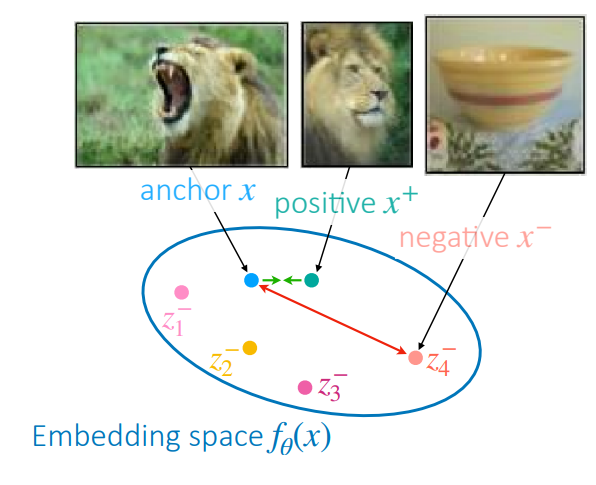
One approach to finding difficult negative samples is called hard negative mining. It essentially just looks through a list of negative samples and tries to see which ones are close your sample in the embedding space. This brings us to the idea of sampling multiple negatives in order to contrast with more difficult negative samples. This is depicted in the figure on the right.

The loss function then becomes an $N$-way classification problem, and it generalizes the triplet loss to using multiple negatives:

\[\mathcal{L}_\mathrm{N-way}(\theta) = -\sum_z \log \left[ \frac{\exp(-d(z, z^+))}{\sum_i\exp(-d(z, z_i^-)) + \exp(-d(z, z^+))} \right]\;.\]

Notice that the goal of this loss is to distinguish the similar sample from all of the negatives with some distance measure of your learned metric space $d(\cdot, \cdot)$, such as a Euclidean loss or negative cosine similarity.

This approach was taken in and , but in practice people often use a slight modification of this loss function, which is shown below:

\[\begin{align*} \mathcal{L}(\theta) &= -\sum_z \log \left[ \frac{\exp(-d(z, z^+))}{\sum_i\exp(-d(z, z_i^-))} \right] \\ &= \sum_z \left[ \exp(-d(z, z^+)) + \log\sum_i\exp(-d(z, z_i^-)) \right]\;. \end{align*}\]

This loss is usually preferred, since you really only want to push away negative examples, not the similar one as well. As you can see in the equivalent formula shown above, this is exactly what it is doing.

The SimCLR algorithm

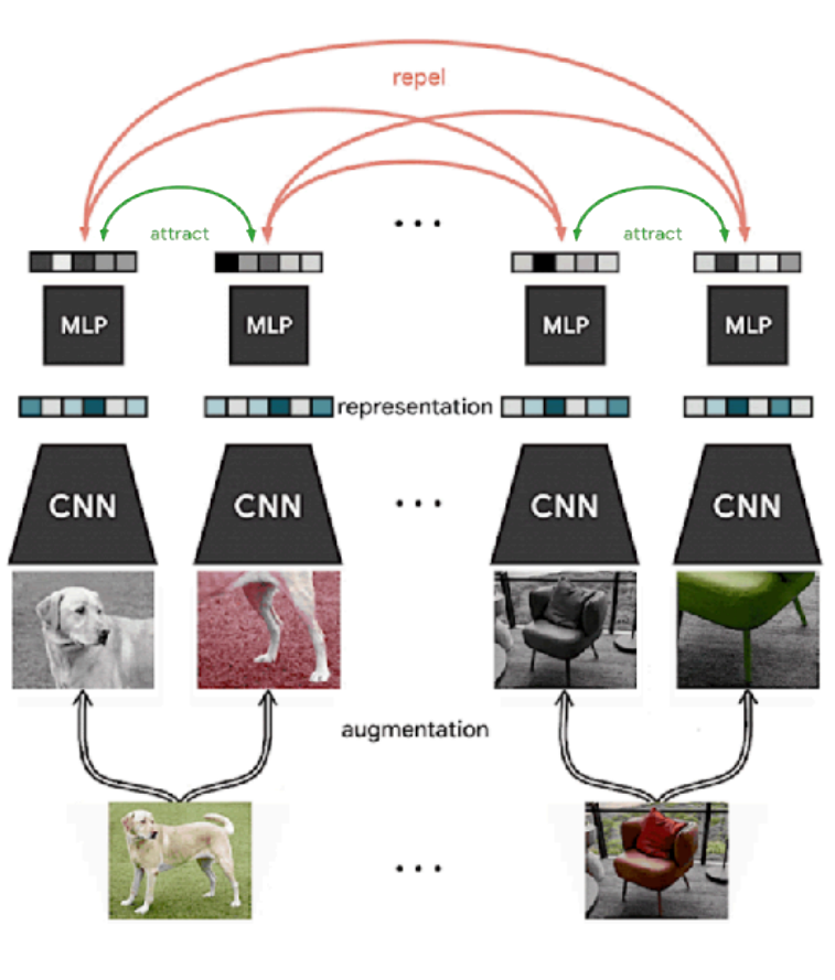
We will now talk about a way of sampling negative examples so we can compute this loss. There is an algorithm called SimCLR which is proposed in , that does exactly this. We visualize this approach in the figure on the right. It is composed of the following steps:

Sample a minibatch of examples $x_1, \cdots, x_N$.
Augment each example twice (design choice) to get $\tilde{x}_1, \cdots, \tilde{x}_N, \tilde{x}_{N+1}, \cdots, \tilde{x}_{2N}$.
Embed examples with $f_\theta$ to get $\tilde{z}_1, \cdots, \tilde{z}_N, \tilde{z}_{N+1}, \cdots, \tilde{z}_{2N}$.
Compute all pairwise distances $d(z_i, z_j) = -\frac{z_i^Tz_j}{\Vert z_i\Vert\Vert z_j\Vert}$ (negative cosine similarity).
Update pairwise distances $\theta$ with respect to $\mathcal{L}_\mathrm{N-way}(\theta)$.

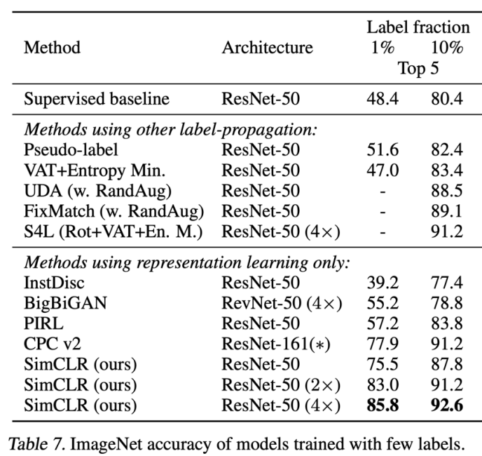
After pre-training the function $f_\theta$, we can either train a classifier on top of the representations that it produces, or choose to fine-tune the entire network. The performance of this method was benchmarked on ImageNet classification, where the model was fine-tuned using only $1$% of all labels (~$12.8$ images per class) or $10$% of all labels. The other part of the dataset was used as unsupervised pre-training data. It shows a substantial improvement over training from scratch, and also improvements over other methods, especially in the $1$% label setting.

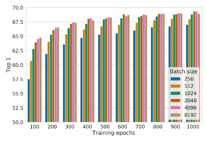
In their experiments, they did note that it was important to use a large batch size (larger than 256), since it leads to longer needed training (more than 600 epochs) in order to get a good performance.

Theoretical properties of contrastive learning

One reason that contrastive learning needs a large batch size, is that the summation over the entire dataset in the $\mathcal{L}_\mathrm{N-way}(\theta)$ loss function will dominate for very close samples. However, if your batch size is too small, you might not include those similar hard examples. This is related to the previous problem of subsampling hard negatives. We will show this mathematically below.

We will rewrite the loss function using a minibatch $\mathcal{B}$ and find a lower bound using Jensen’s inequality:

\[\begin{align*} & \exp(-d(z, z^+)) + \log\sum_n\exp(-d(z, z_n^-)) \\ \geq \: &\exp(-d(z, z^+)) + \sum_{\mathcal{B}} \log\sum_{n \in \mathcal{B}}\exp(-d(z, z_n^-))\;. \end{align*}\]

This shows that our training objective that uses minibatches actually solves a lower bound on the original objective. This means that we might not actually be minimizing our original objective. However, the larger the batch size, the closer the lower bound gets to the original objective function. Can you see why? Answer: We can express $\sum_n = \sum_\mathcal{B}\sum_{n\in\mathcal{B}}$. If you let you minibatch be the entire dataset, then we only have one minibatch, so the $\sum_{\mathcal{B}}$ in the lower bound will disappear and turn into objective function. However, in the worst case with a batch size of 1, we have only one value for $\sum_{n \in \mathcal{B}}$ and many sums over minibatches $\sum_{\mathcal{B}}$, meaning that the lower bound will be the further away from the initial objective.

Recent works in contrastive learning

There are some papers that try to tackle the problem of optimizing this lower bound:

One idea is to store representations from previous batches using a form of momentum during training. It’s not completely correct, but they show it obtains good results with a batch size of $256$ .
It is also possible to predict representations of the same image under different augmentation. In this case, you do not require any negatively similar examples . It’s more of a predictive approach, but does not have a nice contrastive representation.

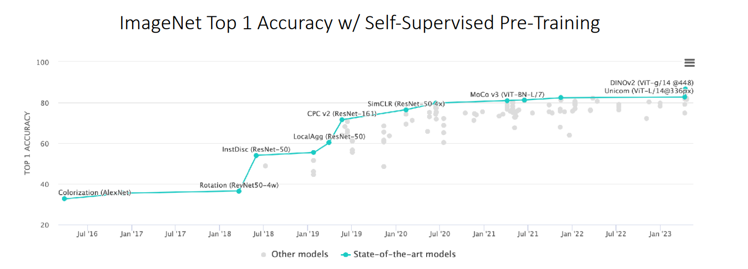
The image above shows results on the ImageNet benchmark over the past years, and contrastive methods (i.e. MoCo v3) are still close to state-of-the-art for self-supervised pre-training for visual data.

In this post we have mainly focussed on augmentation-based methods. However, for many applications, we do not have well-engineered augmentations.

A recent work at ICLR in 2021 tries to learn the augmentations in an adversarial manner. It is competitive with SimCLR on image data and obtains good results on speech and sensor data.
Furthermore, time-contrastive learning on videos has been shown as effective for robotics pre-training, as presented in a paper presented at CoRL in 2022. The method of this paper has been depicted in the figure below.

Process of the time-contrastive learning for robotics pre-training paper.
Finally, the popular CLIP paper uses image-text contrastive pre-training to produce robust zero-shot models. It learns a representation of images and a representation of text, and can tell which images and captions go together (positive samples), and which ones should be pushed apart (negative samples). It shows good zero-shot transfer to out-of-distribution tasks.

Example of how CLIP works and the performance on out-of-distribution tasks.

In summary, contrastive learning is a general and effective framework to do unsupervised pre-trained for few-shot adaptation. It does not require generative modelling and can incorporate domain knowledge through augmentations and similarity. However, it can be difficult to select negative samples, it often requires a large batch size for training, and is currently most successful with augmentations.

Contrastive learning as meta learning

Many of the equations that we saw in this post look similar to the ones that we saw in the previous post about non-parametric meta learning. It is actually possible to create a meta learning algorithm that works similarly to the contrastive approaches that we have seen today. Let’s formulate the problem as a meta learning problem:

Given an unlabelled dataset ${x_i}$.
Create a class $y_i$ from each datapoint via data augmentation $\mathcal{D}_i := \{\tilde{x}_i, \tilde{x}_i^\prime, \cdots\}.$
Run any meta learning algorithm on this dataset.

There is a paper that goes in depth into similarities of SimCLR with Prototypical networks for meta learning, and shows the methods differ in the following ways:

SimCLR samples one task per minibatch, whereas meta learning usually samples multiple.
SimCLR compares all pairs of samples, whereas meta learning compares query examples only to support examples and not to query other examples.

In the table below, they also show that both representations transfer similarly well between different datasets.