CS-330 Lecture 2: Transfer Learning and Meta-Learning
This lecture is part of the CS-330 Deep Multi-Task and Meta Learning course, taught by Chelsea Finn in Fall 2023 at Stanford. The goal of this lecture is to learn how to transfer knowledge from one task to another, discuss what it means for two tasks to share a common structure, and start thinking about meta learning.
The goal of this lecture is to learn how to transfer knowledge from one task to another, discuss what it means for two tasks to share a common structure, and start thinking about meta learning. If you missed the previous lecture, which was about multi-task learning, you can head over here to view it.
As always, since I am still new to this blogging thing, reach out to me if you have any feedback on my writing, the flow of information, or whatever! You can contact me through LinkedIn. ☺
The link to the lecture slides can be found here.
Transfer learning
In contrast to multi-task learning, which tackles several tasks $\mathcal{T}_1, \cdots, \mathcal{T}_i$ simultaneously, transfer learning takes a sequential approach. It focuses on mastering a specific task $\mathcal{T}_b$ after the knowledge has been acquired from source task(s) $\mathcal{T}_a$. A common assumption is that $\mathcal{D}_a$ cannot be accessed during the transfer.
Transfer learning is a valid solution to multi-task learning, because it can sequentially apply knowledge from one task to another. This is unlike multi-task learning, which requires simultaneous learning of all tasks.
It is advantageous in the case of a large dataset $\mathcal{D}_a$, where continuous retraining is not feasible. Transfer learning makes sense here by utilizing the acquired knowledge without the need for repetitive training on the large dataset. Additionally, when you do not need to train two tasks simultaneously, you might opt to solve it them sequentially using transfer learning.
Transfer learning through fine-tuning
\[\phi \leftarrow \theta - \alpha \nabla_\theta \mathcal{L}(\theta, \mathcal{D}_\mathrm{tr})\;.\]One method of transfer learning involves the fine-tuning of a pre-trained model with parameters $\theta$. This process starts with a model whose parameters have been initially trained on a large, diverse dataset, such as ImageNet
When utilizing fine-tuning for transfer learning, there are several common design choices that are usually considered:
- Opting for a lower learning rate to prevent the overwriting of the knowledge captured during pre-training.
- Employing even smaller learning rates for the earlier layers of the network, preserving more generic features.
- Initially freezing the early layers of the model, then gradually unfreezing them as training progresses.
- Reinitializing the last layer to tailor it to the specifics of the new task.
- Searching over hyperparameters using cross-validation to find the optimal configuration.
- Making smart choices about the model architecture.

❗However, this common knowledge does not always hold true. For example, when using unsupervised pre-trained objectives, you may not require diverse data for pre-training. The figure above shows that a model that was pretrained on the downstream dataset performs similarly to an upstream corpus such as BookWiki

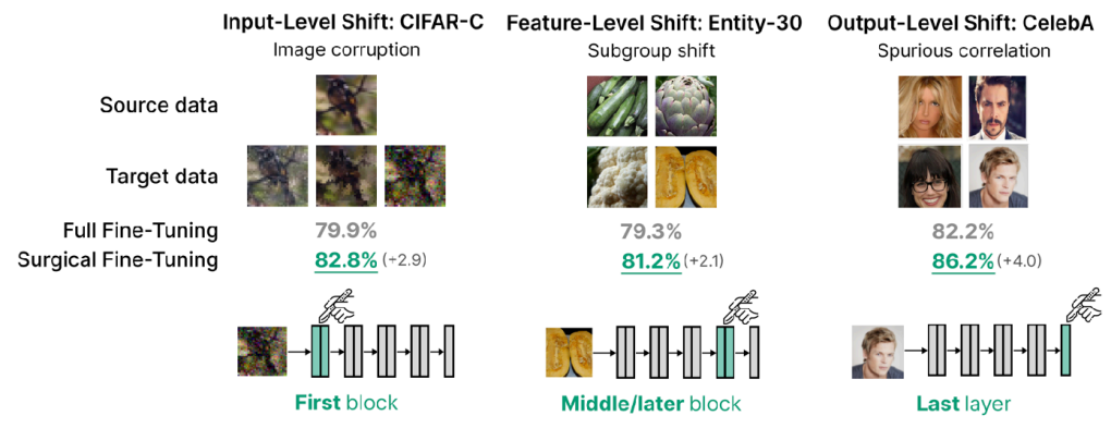
Furthermore, depending on the downstream task, it may be better to tune the first or middle layers, rather than the last layers. For example, for image corruption, it makes more sense to fine-tune the first layer of the model, since it’s more of an input-level shift in data distribution

However, one big disadvantage to fine-tuning is that it does not work well for very small target datasets. An example of this can be seen in the figure above. Luckily, this is where meta learning comes into play!
Introduction to meta learning
With transfer learning, we initialize a model and then hope that it helps to solve the target task, by for example fine-tuning it. With meta-learning, we are asking the question of whether we can explicitly optimize for transferability. Thus, given a set of training tasks, can we optimize the ability to learn these tasks quickly, so that we can learn new tasks quickly too.
When learning a task, we are very roughly mapping a task dataset to a set of model parameters through a function $\mathcal{D}^\mathrm{tr}_i \rightarrow \theta$. In meta learning, we are asking whether we can optimize this function for a small $\mathcal{D}_i^\mathrm{tr}$.
There are two ways to view meta-learning algorithms:
(1) Mechanistic view
Construct a deep network that can read in an entire dataset and make predictions for new datapoints. Training this network uses a meta-dataset, which itself consists of many datasets, each for a different task.
(2) Probabilistic view
Extract shared prior knowledge from a set of tasks that allows for efficient learning of new tasks. Then, learning a new task uses this prior and a (small) training set to infer the most likely posterior parameters.
A probabilistic view on meta learning

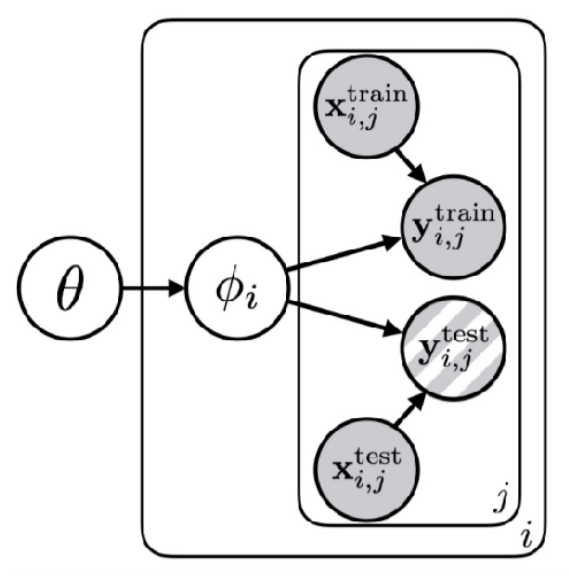
Expanding on the probabilistic (Bayesian) view of meta learning, let’s look at a graphical model for multi-task and meta learning. To quickly recap what a graphical model represents, consider two random variables $X$ and $Y$. If there is an arrow from $X$ to $Y$ in the graphical model, it means that $p(Y\vert X) \neq P(Y)$, meaning that the random variable $Y$ is dependent on $X$. Furthermore, you can nest certain variables (the rounded squared squares with $i$ and $j$) in the figure on the right, if you would like to repeat them for different indices.
Now we can start interpreting the graphical model for multi-task learning. Merging the training and testing sets, we immediately see that the target variable of datapoint $j$ for task $i$, denoted as $y_{i,j}$, is dependent on both the input data $x_{i,j}$ and the task-specific “true” parameter(s) $\phi_i$. The only difference between the training and testing data is that the target variables of the test dataset are not observed, whilst the others are all latent variables (unobserved). As we saw, for each task, we have task-specific true parameters $\phi_i$. However, if we share some common structure between multiple tasks, we can condition these parameters on this common structure. Hence, $\theta$ defines the parameters related to the shared structure between different tasks.
This shared structure means that task parameters $\phi_{i_1}, \phi_{i_2}$ become independent when conditioning on the shared parameters $\theta$: $\phi_{i_1} \perp \phi_{i_2} \vert \theta$. Furthermore, the entropy of $p(\phi_i \vert \theta)$ is lower than $p(\phi_i)$, as there is less distributional noise from common structure.
Let’s now have a thought exercise. If we can identify $\theta$, then when should learning $\phi_i$ be faster than learning from scratch? Let’s think about one extreme. If the shared information fully describes the task-specific information, we would see that $p(\phi_i \vert \theta) = p(\phi_i \vert \phi_i) = 1$. From that, we can see that it is faster if there is a lot of common information about the task that is captured by $\theta$. In a more general case, if the entropy $\mathcal{H}(p(\phi_i\vert\theta)) = 0$, meaning that you can predict $\phi_i$ with 100% accuracy given $\theta$, you can learn the fastest. However, this does not necessarily mean that $\phi_i = \theta$!
From all of this, we can define structure as a statistical dependence on shared latent information $\theta$. Let’s now see some examples of the type of information that $\theta$ may contain.
- In a multi-task sinusoid problem, $\theta$ corresponds to the family of sinusoid functions, which is everything except the phase and amplitude.
- In a multi-language machine translation problem, $\theta$ corresponds to the family of all language pairs.
Note that $\theta$ is narrower than the space of all possible functions!
We will discuss this probabilistic view on meta learning more in later lectures, but for the remainder of this lecture, we will switch back to the mechanistic view.
How does meta learning work?

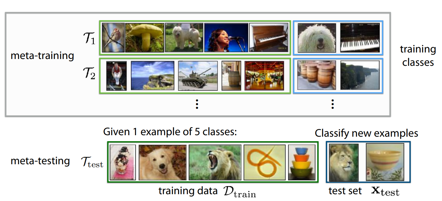
Let’s consider an image classification problem, where you have different tasks. In the problem above, the different tasks contain different images to classify. For the (meta-)training process, we have tasks $\mathcal{T}_1, \mathcal{T}_2, \cdots, \mathcal{T}_n$ and we would like to do meta-testing on a new task $\mathcal{T}_\mathrm{test}$. The goal is to learn to solve task $\mathcal{T}_\mathrm{test}$ more quickly than from scratch. We can then test after training on the few examples from the new (in this case testing) task $\mathcal{T}_\mathrm{test}$. Of course, this problem settings generalizes to any other machine learning problem like regression, language generation, skill learning, etc.
The key assumption here is that meta-training tasks and meta-testing tasks are drawn i.i.d. from the same task distribution $\mathcal{T}_1, \cdots, \mathcal{T}_n,\mathcal{T}_\mathrm{test} \sim p(\mathcal{T})$, meaning that tasks must share structure.
Analogous to more data in machine learning, the more tasks, the better! You can say that meta learning is transfer learning with many source tasks.
The following is some terminology for different things you will hear when talking about meta learning:
- The task-specific training set $\mathcal{D}_i^\mathrm{tr}$ is often referred to as the support set or the context.
- The task test dataset $\mathcal{D}_i^\mathrm{test}$ is called the query set.
- k-shot learning refers to learning with k examples per class.
A general recipe for meta learning algorithms
Let’s formalize meta supervised learning in a mechanistic view. We are looking for a function $y^\mathrm{ts} = f_\theta(\mathcal{D}^\mathrm{tr}, x^\mathrm{ts})$, which is trained on the data $\{\mathcal{D}_i\}_{i=1,\cdots,n}$. This formulation reduces the meta-learning problem to the design and optimization of $f_\theta$.
To approach a problem using meta learning, you will need to decide on two steps:
- What is my form of $f_\theta(\mathcal{D}^\mathrm{tr}, x^\mathrm{ts})$?
- How do I optimize the meta-parameters $\theta$ with respect to the maximum-likelihood objective using meta-training data.
The following lectures will focus on core methods for meta learning and unsupervised pre-trained methods!