CS-330 Lecture 4: Optimization-Based Meta-Learning

This lecture is part of the CS-330 Deep Multi-Task and Meta Learning course, taught by Chelsea Finn in Fall 2023 at Stanford. The goal of this lecture is to understand the basics of optimization-based meta learning techniques. You will also learn about the trade-offs between black-box and optimization-based meta learning!

The goal of this lecture is to understand the basics of optimization-based meta learning techniques. You will also learn about the trade-offs between black-box and optimization-based meta learning! If you missed the previous lecture, which was about black-box meta learning and in-context learning with GPT-3, you can head over here to view it.

As always, since I am still new to this blogging thing, reach out to me if you have any feedback on my writing, the flow of information, or whatever! You can contact me through LinkedIn. ☺

The link to the lecture slides can be found here.

Overall approach

In the previous post, we looked into black-box meta learning. To recap, this approach attempts to output task-specific parameters or contextual information with some meta-model. One major benefit of this approach is its expressiveness. However, it also requires solving a challenging optimization problem, which is incredibly data-inefficient.

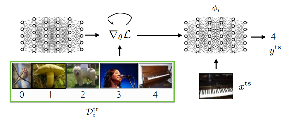
Alt text. — Computation pipeline for optimization-based meta learning.

In this post, we will focus on optimized-based meta learning. The key idea behind this is to embed optimization inside the inner learning process. In the figure above, an example of this idea is depicted. With some initial model $f_\theta$, we will run gradient descent on the datapoints in $\mathcal{D}_i^\mathrm{tr}$ to produce the task-specific network with parameters $\phi_i$. In summary, the goal will be to find the model parameters $\theta$ such that optimizing these parameters to specific tasks is as effective and efficient as possible.

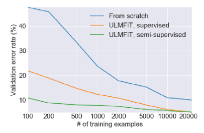
As recalled from a previous post, we are trying to do a similar thing in fine-tuning. Specifically, in fine-tuning, we are using a pre-trained model with parameters $\theta$ to find new task-specific parameters $\phi \leftarrow \theta - \alpha \nabla_\theta \mathcal{L}(\theta, \mathcal{D}^\mathrm{tr})$. We also saw that fine-tuning often performed much better than training from scratch. However, fine-tuning generally needs a lot of data in order to adapt well to a new task, meaning it doesn’t perform well with few-shot learning.

You may now see that our proposed optimization-based meta learning approach tries to optimize pre-trained parameters $\theta$, such that it does well in the few-shot regime, unlike transfer learning through fine-tuning. If we now adapt the meta learning objective function from the previous lecture with this fine-tuning, we obtain the following:

\[\min_\theta \sum_{\mathcal{T}_i}\mathcal{L}(\theta - \alpha \nabla_\theta\mathcal{L}(\theta, \mathcal{D}^\mathrm{tr}_i), \mathcal{D}^\mathrm{test}_i)\;.\]

As you can see in the equation, you are trying to find the parameters $\theta$, such that performing fine-tuning $\theta - \alpha \nabla_\theta\mathcal{L}(\theta, \mathcal{D}^\mathrm{tr}_i)$ on a dataset $\mathcal{D}^\mathrm{tr}_i$ of a task $\mathcal{T}_i$ performs well on the task-specific test set $\mathcal{D}_i^\mathrm{test}$. If these datasets are small, the objective function will still need to optimize pre-training the model for effective fine-tuning on these tasks, meaning that it might work in the few-shot regime.

We can write down the general training pipeline with the following steps:

Sample a task $\mathcal{T}_i$.
Sample disjoint datasets $\mathcal{D}_i^\mathrm{tr}$ and $\mathcal{D}_i^\mathrm{test}$ from $\mathcal{D}_i$.
Optimize $\phi_i \leftarrow \theta - \alpha \nabla_\theta\mathcal{L}(\theta, \mathcal{D}_i^\mathrm{tr})$.
Update $\theta$ using $\nabla_\theta \mathcal{L}(\phi_i, \mathcal{D}_i^\mathrm{test})$.

Notice that we only optimize $\phi_i$ to then use it to update parameters $\theta$. This means that $\phi_i$ is discarded and re-computed at each iteration. Additionally, we can optimize for different parameters, such as $\alpha$ as well by including it as a parameter in $\theta$. Besides computational efficiency of this, there is another problem. If we expand $\nabla_\theta \mathcal{L}(\phi_i, \mathcal{D}_i^\mathrm{test})$, we get second-order derivates. Let’s show this below:

\[\begin{align*} \nabla_\theta\mathcal{L}(\phi_i, \mathcal{D}_i^\mathrm{test}) &= \nabla_{\bar{\phi}}\mathcal{L}(\bar{\phi}, \mathcal{D}_i^\mathrm{test})\bigg|_{\bar{\phi} = \phi_i} \frac{\partial\phi_i}{\partial\theta} \\ &= \nabla_{\bar{\phi}}\mathcal{L}(\bar{\phi}, \mathcal{D}_i^\mathrm{test})\bigg|_{\bar{\phi} = \phi_i}\left(I - \alpha \nabla^2_\theta\mathcal{L}(\theta, \mathcal{D}^\mathrm{tr}_i)\right)\;. \end{align*}\]

Unfortunately, we can see the Hessian $\nabla^2_\theta\mathcal{L}(\theta, \mathcal{D}^\mathrm{tr}_i)$. We would have to compute this, but luckily, $\nabla_{\bar{\phi}}\mathcal{L}(\bar{\phi}, \mathcal{D}_i^\mathrm{test})\vert_{\bar{\phi} = \phi_i}$ is a row vector. Due to Hessian-vector products, we can compute $\nabla_\theta\mathcal{L}(\phi_i, \mathcal{D}_i^\mathrm{test})$ without computing the whole Hessian. Let’s show this below:

\[\begin{align*} g(x + \Delta x) &\approx g(x) + H(x)\Delta x \\ g(x + rv) &\approx g(x) + rH(x)v \\ H(x)v &\approx \frac{g(x+rv) - g(x)}{r}\;. \end{align*}\]

In the first line, we are using a simple Taylor expansion to approximate the function $g(x+\Delta x)$, which is the gradient function. Then, we rewrite $\Delta x$ as with scalar $r$ and vector $v$. We can finally rearrange the equation to get to our result. The last line shows that we can approximate a Hessian-vector product by using two gradient evaluations. Whilst this is still more than one, it is much more computationally efficient than computing the entire Hessian matrix.

Since $\nabla_{\bar{\phi}}\mathcal{L}(\bar{\phi}, \mathcal{D}_i^\mathrm{test})\vert_{\bar{\phi} = \phi_i}\left(I - \alpha \nabla^2_\theta\mathcal{L}(\theta, \mathcal{D}^\mathrm{tr}_i)\right) = v -\alpha vH$, you can see that we can use the previous result to compute the gradient, rather then computing the whole Hessian.

A common misconception is that you will get higher than 2nd-order derivatives when computing multiple iterations of $\phi_i \leftarrow \theta - \alpha \nabla_\theta\mathcal{L}(\theta, \mathcal{D}_i^\mathrm{tr})$. However, this is not true, since the derivatives will be sequential rather than nested. You can try this yourself if you want to test your knowledge! If you do this correctly, you will see that doing more iterations will increase the amount of memory used linearly, and the amount of compute necessary linearly as well. In practice, usually you do not need more than 5 inner gradient steps, which is usually fine for few-shot learning tasks. In future posts, we will discuss methods that work for hundreds of inner gradient steps.

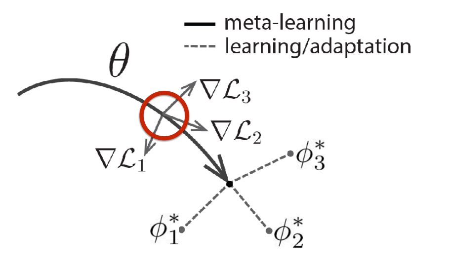
This approach, which is called Model-Agnostic Meta-Learning (MAML), is also represented in the figure on the right. Here, $\phi_1^*, \phi_2^*, \phi_3^*$ are the optimal parameters for tasks $1, 2, 3$.

At meta-test time, we can follow the following steps, which are very similar to meta-training:

Sample a task $\mathcal{T}_i$.
Given training dataset $\mathcal{D}_j^\mathrm{tr}$.
Optimize $\phi_j \leftarrow \theta - \alpha \nabla_\theta\mathcal{L}(\theta, \mathcal{D}_j^\mathrm{tr})$.
Make predictions on new datapoints $f_{\phi_j}(x)$.

Compare: optimization-based vs. black-box

In the previous section, we got some intuition behind the Model-Agnostic Meta-Learning algorithm. For now, it looks like this method is completely different from black-box meta learning, but let’s spend some times trying to understand the connection between the two. Let’s write down both objectives again.

Black-box meta learning

$y^\mathrm{ts} = f_\mathrm{black-box}(\mathcal{D}^\mathrm{tr}_i, x^\mathrm{ts})$.

Model-agnostic meta learning (MAML)

$y^\mathrm{ts} = f_\mathrm{MAML}(\mathcal{D}^\mathrm{tr}_i, x^\mathrm{ts}) = f_{\phi_i}(x^\mathrm{ts})$, where $\phi_i = \theta - \alpha \nabla_\theta \mathcal{L}(\theta ,\mathcal{D}_i^\mathrm{tr})$.

If you look at both equations, both equations look more similar than it may seem. Both methods are still only functions of $\mathcal{D}^\mathrm{tr}_i$ and $x^\mathrm{ts}$. The main difference is that MAML uses an “embedded” gradient operator in its computation graph, which is just a directed graph of all computations that is done by the function.

Keeping this idea of a computation graph in mind, you might think of the idea to mix and match different components of the computation graph. This idea has been explored in various works. For example, one paper learned the initialization parameters $\theta$, but replaced the gradient updates with a learned network, meaning that $\phi_i = \theta - f(\theta, \mathcal{D}_i^\mathrm{tr}, \nabla_\theta\mathcal{L})$. It turns out this approach is not very practical, but it has a nice conceptual meaning that goes along well with the idea of a computation graph.

Comparing performances

We now wish to compare the two different approaches to each other. First, let’s think about the following: If we have a test task $\mathcal{T}_j$ that is a bit different from the tasks that we trained our models on, which approach do you think will be better?

We hope to see that optimization-based meta learning performs better in this case, because it’s explicitly optimizing the effectiveness of fine-tuning to new tasks. With black-box meta learning, we are essentially just training a model to output model parameters or context, which does not guarantee to work for unseen tasks (though we hope it will!).

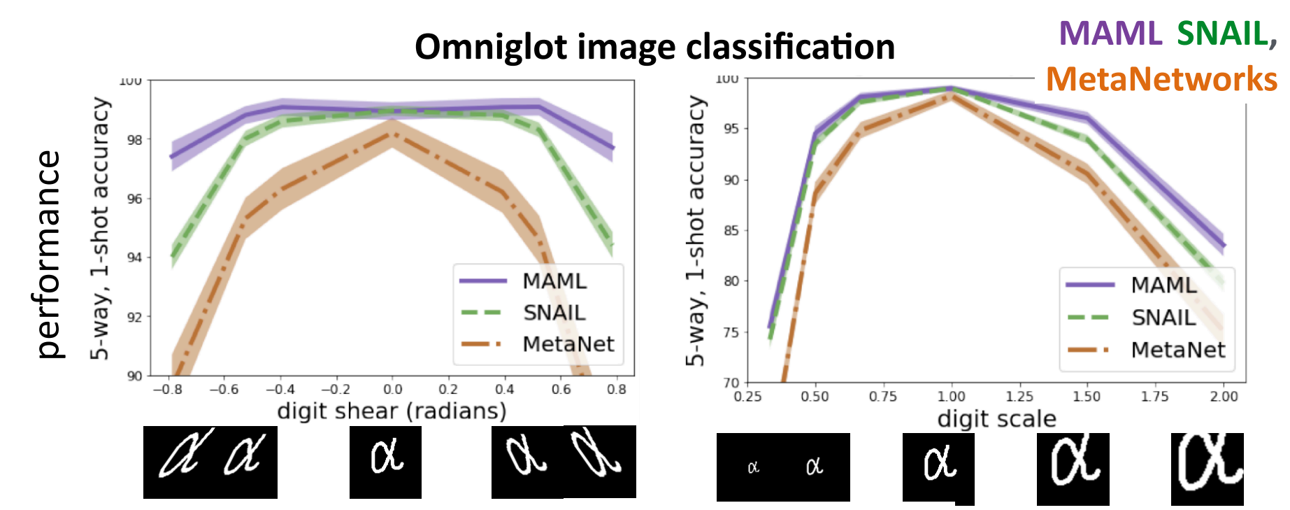
We will test this by looking at the Omniglot image classification problem again. However, we will try to see what happens when we vary the tasks after training the models on them. In this case, digits from the datasets are warped to see a form of out-of-distribution performance. In the figure above, which is taken from, you can see that, as expected, an optimization-based method like MAML performs much better than black-box-based approaches like SNAIL or MetaNet for these types of problems.

You might think that this structure comes at a cost of expressiveness. But, in , they showed that MAML can approximate any function of $\mathcal{D}^\mathrm{tr}_i, x^\mathrm{ts}$ given some assumptions (i.e. you need a very deep network for this to hold). However, despite these assumptions, this result shows that MAML benefits of the inductive bias of optimizing fine-tuning explicitly without losing any of the expressive power.

Challenges and solutions

Whilst optimization-based meta learning methods may sound perfect from this post, there are quite some challenges when using these methods. We will list some of them and discuss them in more detail.

Bi-level optimization can exhibit instabilities.

This can be the case because you have nested optimizations that are heavily dependent on each other. Some unexpected result in one level of the optimization can result in an unexpected effect, which will then be propagated throughout training. There are multiple simple tricks that can be used to try to stabilize training:
- Automatically learn inner vector learning rate, tune outer learning rate .
- Optimize only a subset of the parameters in the inner loop .
- Decouple inner learning rate, batch normalization statistics per-step .
- Introduce context variables for increased expressive power .
Backpropagating through many inner gradient steps is compute- & memory-intensive.

As we said before, the amount of inner gradient steps with MAML is usually only around 5, due to the amount of compute and memory required to optimize over such a computation graph. Again, there are some tricks to try to address this, but we will discuss more options in the lecture about large-scale meta learning.
- (Crudely) approximate $\frac{\delta\phi_i}{\delta\theta}$ as the identity matrix . This seems to work surprisingly well for simple few-shot learning problems, but it doesn’t scale to more complex problems.
- Only optimize the last layer of weights using ridge regression, logistic regression , or support vector machines . This can lead to a closed form convex optimization problem on top of the meta-learned features.
- Derive the meta-gradient using the implicit function theorem . This way you can compute the full gradient without differentiating through the entire computation graph of the multiple iterations.

Let’s summarize the upsides and downsides:

Upsides

Positive inductive bias at the start of meta learning.
Extrapolates better via structure of optimization.
Maximally expressive for a sufficiently deep network.
Model-agnostic!

Downsides

Typically requires second-order optimization.
Can be compute and/or memory intensive.
Can be prohibitively expensive for large models.

Case study of land cover classification

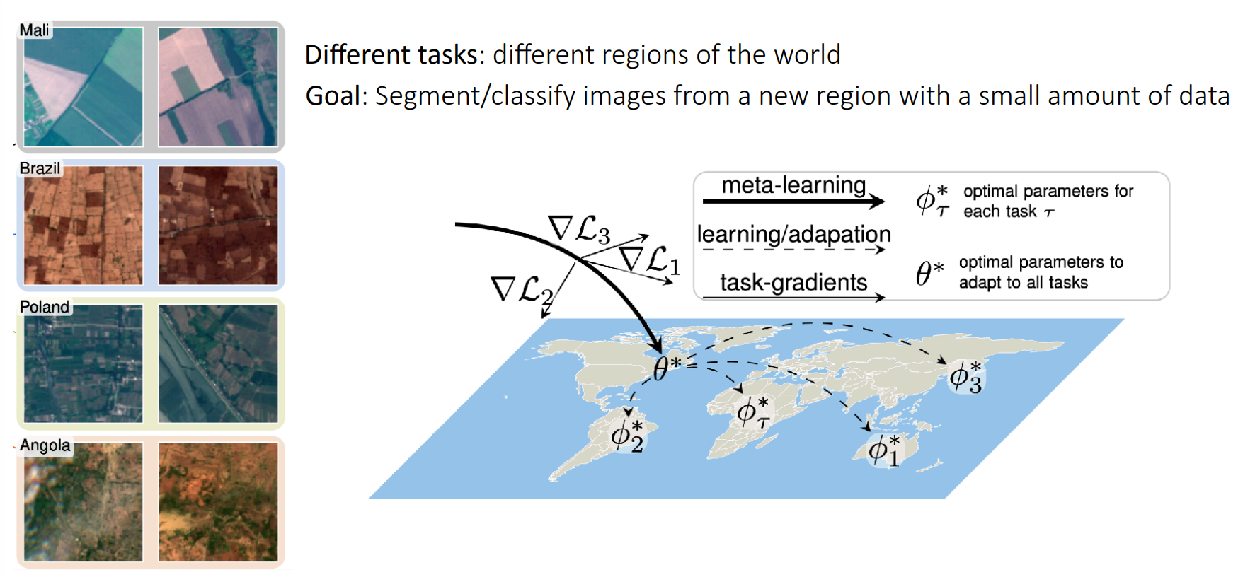
We will now study an example of optimization-based meta learning for a pretty cool problem: land cover classification ! Imagine that you are given a bunch of satellite data of different terrains, and your goal is to predict what the land is used for by segmenting it into different classes. Research like this can for example be used to understand how different climates change over time, or urban planning. Unfortunately, it is very expensive to label these images, leading to small datasets.

As you can see in the image above, we have terrains from different regions of the world, which can look very different, but probably still share some geological structural similarities. Given this description, try to think to yourself: Do you think meta learning would be a good approach to this problem?

If we let our tasks correspond to these different regions, we can try to use optimization-based meta learning to learn to effectively and efficiently fine-tune to unknown regions of the world! For these new regions, we would manually segment small amount of data, and then use our model to take care of the rest.

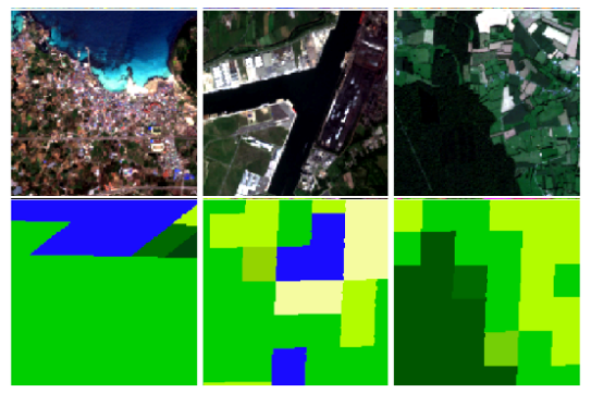
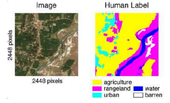
The paper looks at two datasets:

SEN12MS , which contains geographic metadata, making it easy to construct good meta-train, meta-val, and meta-test sets.

DeepGlobe , which did not provide this metadata. Instead, clustering was used to create datasets of similar terrains.

The results of using MAML on these two datasets is shown in the figure above. As you can see, MAML is more efficient and effective than (dark blue) pre-training on meta-training data and fine-tuning and (light blue) training on the new terrain from scratch. Hopefully these results give you a good idea of the potential of meta learning for few-shot learning!