CS-330 Lecture 1: Multi-Task Learning
This is the first lecture of the CS-330 Deep Multi-Task and Meta Learning course, taught by Chelsea Finn in Fall 2023 at Stanford. The goal of this lecture is to understand the key design decisions when building multi-task learning systems.
The goal of this lecture is to understand the key design decisions when building multi-task learning systems. Since I am still new to this blogging thing, reach out to me if you have any feedback on my writing, the flow of information, or whatever! You can contact me through LinkedIn. ☺
The link to the lecture slides can be found here.
Problem statement
We will first establish some notation that will be used throughout the course. Let’s first introduce the single-task supervised learning problem.
\[\min_\theta \mathcal{L}(\theta, \mathcal{D}), \quad \text{s.t.} \quad \mathcal{D} = \{(x,y)_k\}\;.\]Here, $\mathcal{L}$ is the loss function, $\theta$ are the model parameters and $\mathcal{D}$ is the dataset. A typical example of a loss function would be the negative log-likelihood function $\mathcal{L}(\theta, \mathcal{D}) = - \mathbb{E}\left[\log f_\theta(y\vert x)\right]$.
We can formally define a task as follows:
\[\mathcal{T}_i := \{p_i(x), p_i(y\vert x), \mathcal{L}_i\}\;.\]Here, $p_i(x)$ is the input data distribution, $p_i(y\vert x)$ is the distribution of the target variable(s), and $\mathcal{L}_i$ is a task-specific loss function (can of course be the same for different tasks). The corresponding task datasets are $\mathcal{D}_i^\mathrm{tr} := \mathcal{D}_i$ and $\mathcal{D}_i^\mathrm{test}$.
Some examples of tasks:
- Multi-task classification ($\mathcal{L_i}$ the same for each task)
- Per-language handwriting recognition.
- Personalized spam filter.
- Multi-label learning ($\mathcal{L_i}$ and $p_i(x)$ the same for each task)
- Face attribute recognition.
- Scene understanding.

It is important to realize that $\mathcal{L}_i$ might change across tasks, for example when mixing discrete from continuous data or if there are multiple metrics that you care about.
Models, objectives, optimization
One way of helping a model identify different tasks would be to condition the model function by a task descriptor $z_i$: $f_\theta(y\vert x, z_i)$. This could be anything ranging from user features, language descriptions, or formal task specifications. The next subsections will focus on how to condition the model, which objective should be used, and how the objective should be optimized.
Model
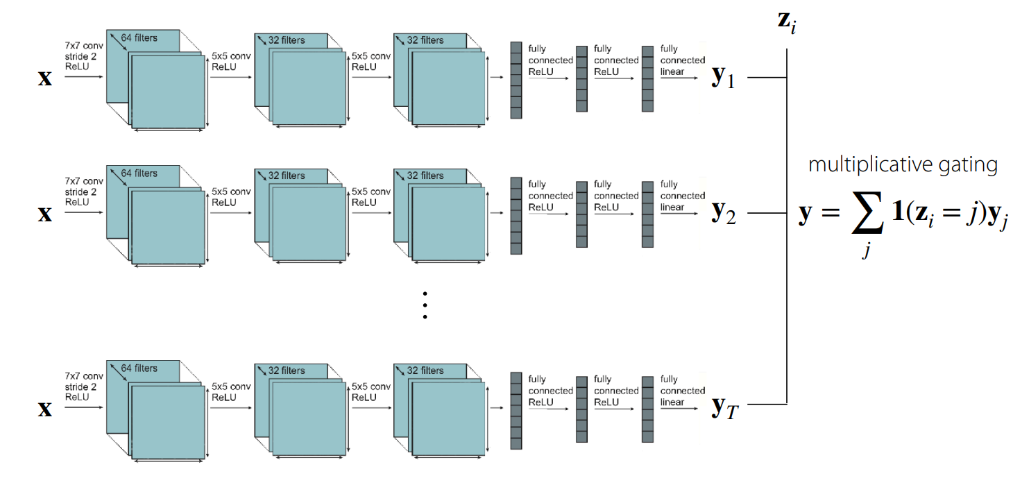
Let’s first think about how we can condition on the task in order to share as little information as possible. The answer to this is simple: you can create a function that uses multiplicative gating with a one-hot encoding of the task . The model function would be $f_\theta(y \vert x, z_i) = \sum_j \mathbb{1}(z_i=j)f_{\theta_i}(x)$. This results in independent training with a single network per tasks; there are no shared parameters. This can be seen in the figure above.
On the other extreme, you could simply concatenate $z_i$ with the input and/or activations in the model. In this case, all parameters are shared (except the ones directly following $z_i$, in case it is one-hot).
This give rise to a question: can you phrase the multi-task learning objective parameters $\theta = \theta_\mathrm{sh} \cup \theta_i$, where $\theta_\mathrm{sh}$ are shared parameters and $\theta_i$ are task-specific parameters? Our objective function becomes the following:
\[\min_{\theta_\mathrm{sh}, \theta_1, \cdots, \theta_T} \sum_{i=1}^T \mathcal{L}_i(\theta_\mathrm{sh} \cup \theta_i, \mathcal{D}_i)\;.\]In this case, choosing how to condition on $z_i$ is equivalent to choosing how and where to share model parameters. We will now look into some basic ways to condition a model.
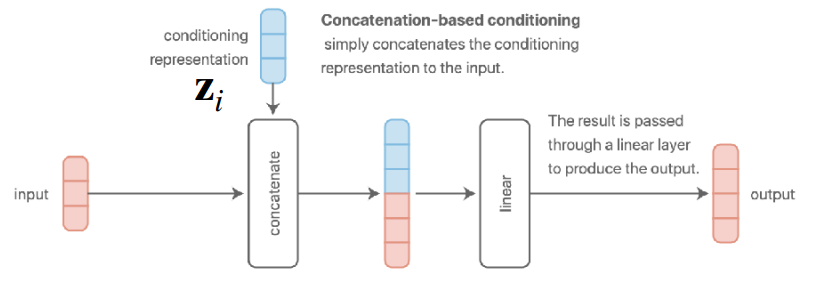
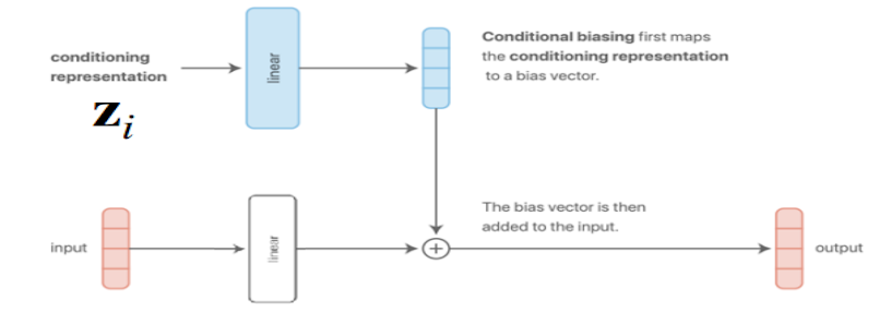
Can you see why additive conditioning in this way is equivalent to concatenation-based conditioning? Hint: think about how matrix multiplication splits the parameters when concatenating
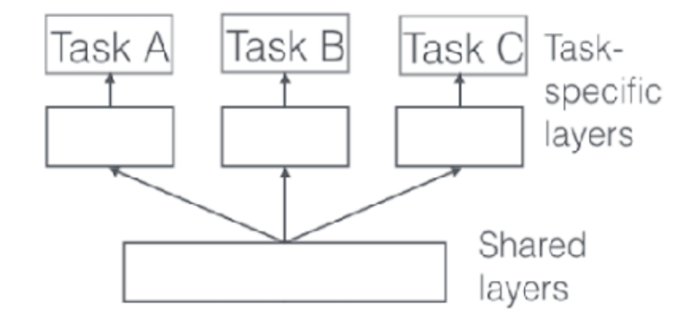
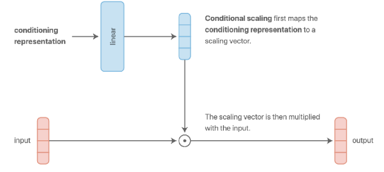
One benefit of multiplicative conditioning is that you have this multiplicative gating, allowing more expressiveness per layer. It generalizes independent networks and independent heads.
There are more complex conditioning techniques, and a lot of research has gone into this topic, such as Cross-Stitch Networks
Unfortunately, these design choices are problem dependent, largely guided by intuition or knowledge about the problem, and currently more of an art than a science.
Objectives
We already saw a previous example of a multi-task objective function. Let’s start with the vanilla multi-task learning (MTL) objective: $\min_\theta \sum_{i=1}^T \mathcal{L}_i(\theta, \mathcal{D_i})$. Let’s now show some other ways to construct multi-task objective functions.
-
Weighted multi-task learning (manually based on priority or dynamically adjust weights throughout training):
\[\min_\theta \sum_{i=1}^T w_i \mathcal{L}_i(\theta, \mathcal{D_i})\;.\] -
Minimax multi-task learning to optimize for the worst-case task loss (useful in robustness or fairness):
\[\min_\theta \max_i \mathcal{L}_i(\theta, \mathcal{D_i})\;.\] -
You can use various heuristics to construct your objective function. One example is to encourage gradients to have similar magnitudes across tasks.
Optimization
For the vanilla MTL objective, a basic training approach follows the following steps:
- Sample mini-batch of tasks $\mathcal{B} = {\mathcal{T}_i}$.
- Sample mini-batch of datapoints for each task $\mathcal{D}^b_i \sim \mathcal{D}_i$.
- Compute mini-batch loss $\hat{\mathcal{L}}(\theta, \mathcal{B}) = \sum_{\mathcal{T}_k \in \mathcal{B}} \mathcal{L}_k(\theta, \mathcal{D}_k^b)$.
- Backpropagate the loss to compute $\nabla_\theta \hat{\mathcal{L}}$.
- Perform a step of gradient descent with some optimizer.
- Repeat from step 1.
This process ensures that tasks are sampled uniformly, regardless of data quantities. However, it is important to ensure that the task labels, and the loss function, are on the same scale.
Challenges
There are multiple challenges that come with multi-task learning.
-
Negative transfer: Sometimes independent subnetworks work better than parameter sharing. This could be due to optimization challenges (cross-task interference or tasks learning at different rates), or limited representational capacity (multi-task networks often need to be much larger than their single-task counterparts).
In the case of negative transfer, you should share less across tasks. You can also add a regularization term to the objective function, to allow soft parameter sharing:
\[\min_{\theta_\mathrm{sh}, \theta_1, \cdots, \theta_T} \sum_{i=1}^T \mathcal{L}_i(\theta_\mathrm{sh} \cup \theta_i, \mathcal{D}_i) + \lambda \sum_{i^\prime = 1}^T \left\Vert \theta_i - \theta_i^\prime \right\Vert\;.\]This allows for more fluid degrees of parameters sharing. However, it does add another set of hyperparameters, and it more memory intensive.
- Overfitting: You might not be sharing enough parameters. Since multi-task learning is equivalent to a form of regularization, the solution could be to share more parameters.
- Having many tasks: You might wonder how to train all tasks together and which ones will be complementary. Unfortunately, no closed-form solution exists for measuring task similarity. Nevertheless, there are ways to approximate it from one training run
.
Case study of real-world multi-task learning
In this case study, we will discuss the paper “Recommending What Video to Watch Next: A Multitask Ranking System”
The framework is constructed as follows:
- Inputs: What the user is currently watching (query video) and user features
The procedure is the following:
- Generate a few hundred of candidate videos (by pooling videos from multiple candidate generation algorithms such as matching topics of the query video, videos frequently watched with the query video, and others).
- Rank the candidates.
- Serve the top ranking videos to the user.
The central topic of this paper is the ranking system. The authors decide that the inputs to the ranking model are the query video, candidate video, and context features. The model attempts to output a weighted combination of engagement and satisfaction predictions, which results in a ranking score. The score weights are manually tuned.
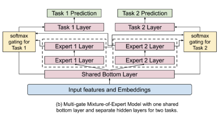
On choice for the model architecture is a “shared-bottom model”, which has some shared bottom layers which split into separate heads for each task. However, this will harm learning when the correlation between tasks is low. Instead, they opt for a form of soft-parameter sharing that they call Multi-gate Mixture-of-Experts (MMoE). As you can see in the figure, this architecture allows different parts of the network to “specialize” in certain tasks as experts. For each task, an attention-like score is computed that decides which combination of experts should be used.
Formally, let’s call the expert networks $f_i(x)$. We then decide which expert to use for input $x$ and task $k$ by computing $g^k(x) = \mathrm{softmax}(W_{g^k}x)$. The features are then computed from the selected experts as $f_k(x) = \sum_{i=1}^n g_{(i)}^k(x)f_i(x)$. The output can finally be denoted by $y_k = h^k(f^k(x))$.
In the paper, they trained them model in temporal order, running training continuously to consume newly arriving data. They perform online A/B testing in comparison to the production system based on some live metrics, and stress that model computational efficiency matters.
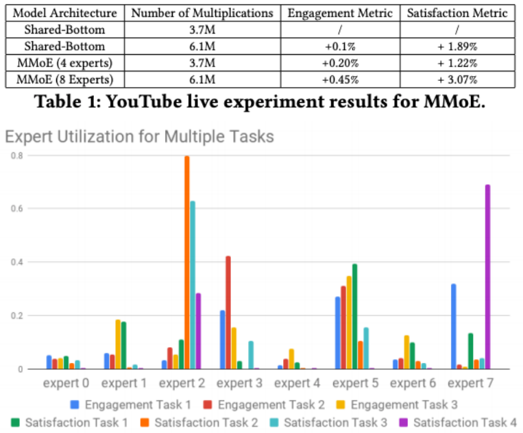
From the results, you can see that this sort of architecture definitely helps. Furthermore, they found that there was a 20% change of gating polarization during distributed training. This means that not all experts are utilized equally and there is a bias to some expert(s). They utilized drop-out on the experts to counteract this problem.