CS-330 Lecture 3: Black-Box Meta-Learning & In-Context Learning

This lecture is part of the CS-330 Deep Multi-Task and Meta Learning course, taught by Chelsea Finn in Fall 2023 at Stanford. The goal of this lecture is to learn how to implement black-box meta-learning techniques. We will also talk about a case study of GPT-3!

The goal of this lecture is to learn how to implement black-box meta-learning techniques. We will also talk about a case study of GPT-3! If you missed the previous lecture, which was about transfer learning by fine-tuning and meta learning, you can head over here to view it.

As always, since I am still new to this blogging thing, reach out to me if you have any feedback on my writing, the flow of information, or whatever! You can contact me through LinkedIn. ☺

The link to the lecture slides can be found here.

Black-box adaptation approaches

Alt text. — Example of the Omniglot dataset.

The content of this section will build on the general recipe for meta-learning problems that we saw in the previous lecture. In order to explain it, we will use the example of the Omniglot dataset , which is a dataset of 1,623 characters from 50 different alphabets. In this problem, every alphabet would refer to a different task. In our example, we will do 3-way 1-shot learning, meaning that our sampled datasets consist of 3 classes with 1 example per class at every step. One iteration of the black-box meta-training process then has the following steps:

Sample task $\mathcal{T}_i$ or a mini-batch of tasks. In our case, this would correspond to generating the language(s).
From the selected language(s), we sample disjoint datasets $\mathcal{D}_i^\mathrm{tr}$ and $\mathcal{D}_i^\mathrm{test}$ from $\mathcal{D}_i$. In our example, this will be a disjoint dataset with 3 samples of characters for every language alphabet.

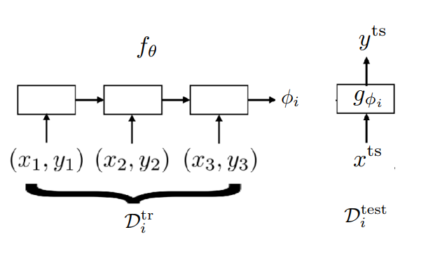
Now that we have these datasets, our goal is to train a neural network to represent $\phi_i = f_\theta(\mathcal{D}_i^\mathrm{tr})$. After computing these task parameters given a sampled training dataset, we can predict the test targets with $y^\mathrm{ts} = g_{\phi_i}(x^\mathrm{ts})$. An example of how such a model could work, is depicted in the figure above. Here, we are using a sequence model for $f_\theta$, which generates the parameters $\phi_i$. However, you can use all your fancy architectures that can handle a varying number of input sample. This is necessary due to varying dataset lengths.

After computing $y^\mathrm{ts}$, we can do backpropagation of the loss that is generated with the this test dataset. The full optimization objective is shown in the equation below:

\[\min_\theta \sum_{\mathcal{T}_i} \sum_{(x,y) \sim \mathcal{D}^\mathrm{test}_i} - \log g_{\phi_i}(y\vert x) = \min_\theta \sum_{\mathcal{T}_i}\mathcal{L}(f_\theta(\mathcal{D}^\mathrm{tr}_i), \mathcal{D}^\mathrm{test}_i)\;.\]

Notice that we are optimizing the parameters $\theta$. The task-specific parameters $\phi_i$ are generated by $f_\theta(\mathcal{D}_i^\mathrm{tr})$, and so they are not updated. Also note that the loss is calculated with respect to the sampled test dataset! This is no problem, since it makes sense to evaluate on new tasks for meta learning.

Now that you understand the architecture, we can write down the last two steps of the meta-training process:

Compute $\phi_i \leftarrow f_\theta(\mathcal{D}_i^\mathrm{tr})$.
Update $\theta$ using $\nabla_\theta \mathcal{L}(\phi_i, \mathcal{D}_i^\mathrm{test})$.

A more scalable architecture

However, we run into an issue. How do we let the model $f_\theta$ output another model’s parameters $\phi_i$? Not only can this be quite tricky to do, it also does not scale to larger parameter vectors $\phi_i$! Can you think of an alternative way of going this?

Instead of letting $f_\theta$ output $\phi_i$, we instead output a hidden state $h_i$, which is a low-dimensional vector that is supposed to represent contextual task information from the training dataset. If you recall the different ways of conditioning that we saw for multi-task learning, you can see that we can train a model end-to-end by conditioning as $y^\mathrm{ts} = g_{\phi}(x^\mathrm{ts} \vert h_i)$. Now, notice that we have a general set of parameters $\phi$ for $g$; it does not need to be task-specific anymore, since we are already conditioning on task information. In the figure above, $\theta$ are the parameters of the sequence model, and $\phi$ are the parameters of the convolutional network.

❗One problem that sometimes occurs with this architecture, is that the model learns to ignore conditioning on $h_i$. In that case, it is essentially just learning to memorize, and not using the training dataset. In order to avoid that, you can randomize the numerical label assignment to the target variables when sampling the datasets $\mathcal{D}^{tr}_i$ and $\mathcal{D}^{test}_i$. If the numerical label is different each time, it cannot just memorize the sample from the testing set.

Black-box adaptation architectures

The architecture that we just presented was more-or-less first proposed on the Omniglot dataset at ICML in 2016 . It used LSTMs with Neural Turing Machines (which are not used anymore nowadays). Since then, a lot of new architectures have been proposed.

At ICML 2018, an architecture called the DeepSet architecture was published. The idea is to pass all your dataset samples through a feedforward neural network to get an embedding of each sample, and then average those. This way, you have a permutation-invariant model which is still model-agnostic. Given some conditions on the width and depth of the network, these models can represent any permutation-invariant function.

There are quite some more papers that used other external memory mechanisms , or convolutions and attention .

Unfortunately, these models are still quite limited in capabilities against “difficult” datasets, as you can see in the table below.

In summary, some benefits of black-box meta learning are its expressiveness, how easy it is to combine with a variety of learning problems (such as SL or RL). Nonetheless, it is a challenging optimization problem for a complex model, and it is often data-inefficient.

Case study of GPT-3

With the rise of research on in-context learning, especially with foundation models, GPT-3 is a good example of a black-box meta-learner, trained on language generation tasks. We can represent the task-specific datasets $\mathcal{D}_i^\mathrm{tr}$ as a sequence of characters, and $\mathcal{D}_i^\mathrm{test}$ as the following sequence of characters. This way, $\mathcal{D}_i^\mathrm{tr}$ is what the model is being conditioned on (its context), and $\mathcal{D}_i^\mathrm{test}$ is what it has to generate.

The meta-training dataset consists of crawled data from the internet, English-language Wikipedia, and two books corpora, with a giant Transformer architecture as its network (175 billion parameters, 96 layers, 3.2M batch size).

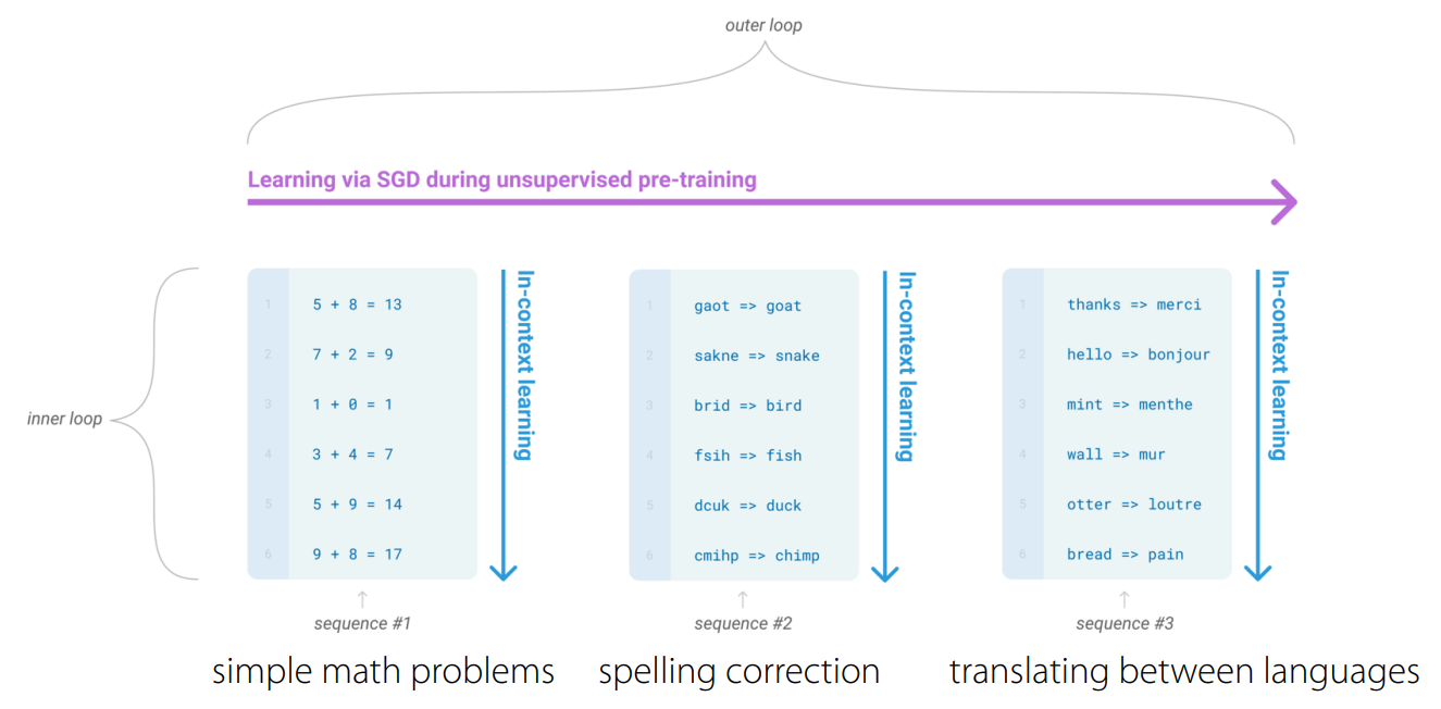
For these datasets, there are a multitude of different tasks such as, but definitely not limited to, spelling correction, simple math problems, or translating between languages. By encoding every task as text, the authors are able to obtain meta-training data incredibly easily.

In the case of GPT-3, text generation, also known as in-context learning, represents the inner loop of the optimization process. The outer loop represents the model optimizing across different tasks, which is very similar to the process that we saw in the previous section.

With this model, you can easily do few-shot learning by adding examples in text form to the context of the model. Even through the model is far from perfect, its results are extremely impressive. It is also no oracle and can fail in unintuitive ways! If there is anything we have learned from recent research, it is that the choice of $\mathcal{D}^\mathrm{tr}$ at test time matters (welcome to the world of prompt engineering).

It is also interesting to think about what is needed for few-shot learning to emerge when training a model. This is an active research are, but it seems that (1) temporal correlation in your data with dynamic meaning of words, and (2) large model capacities definitely seems to make a difference here .